Does a Rainfall Total Tell You How Hard It Rained?

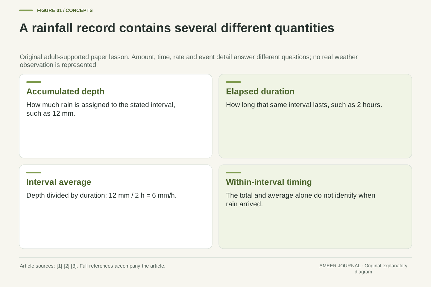
A weather card says twelve millimetres of rain fell in two hours. Was the rain steady, or did most of it arrive in a short shower? The total alone cannot tell us. Rain accumulation describes how much arrived over a period. Rain rate describes how quickly it arrived. The Met Office explains these as different weather measurements [2].

We can still work out something useful: the average over those two hours is six millimetres per hour. That is a way of sharing the total across the whole interval. It does not mean that each hour, minute or second actually received an equal share. To learn about those smaller periods, we would need more detailed records.

Explore the invented cards and diagrams with an adult, on screen or on uncut paper. No outdoor weather watching, rain collection, containers, glass, tools or water are needed. There is no storm to investigate and nothing to upload. Our numbers are a paper lesson about measurement, not observations from a real place or predictions about tomorrow.

Rainfall accumulation and rainfall rate answer different questions. The Met Office distinguishes accumulation over an interval from the speed at which precipitation is arriving [2]. An accumulated depth, its start and end times, and an instantaneous or shorter-window rate should therefore remain separate fields when interpreting a weather record.

This article uses explicitly invented examples to examine the information retained by different records. A depth of twelve millimetres over two hours defines a six-millimetre-per-hour interval average. It does not determine a unique time-varying rate. Later examples distinguish a gauge's nominal event credits from physical input when an unfinished increment remains inside the measurement mechanism.

The activity is private, adult-supported reading, pointing or drawing on uncut paper. No actual weather observation, gauge experiment, outdoor activity, water handling, tools, glass, location collection or child submission is involved. The calculations establish properties of the stated records and idealized mechanisms; they do not classify weather hazards, validate a particular instrument or issue a forecast.

A rainfall depth is a way to describe an amount without confusing it with the size of the collecting opening. Imagine rain spread evenly over two imaginary, level openings. If both receive a depth of four millimetres, the larger opening catches more water. The depth can be the same even though the collected volumes differ. Actual gauge descriptions identify the collector's sampling area [1][4].

Give the first opening an area of one hundred square centimetres and the second fifty. Four millimetres is 0.4 centimetres. In our perfect collection example, area multiplied by depth gives forty cubic centimetres of water for the first opening and twenty for the second. Twice the opening area receives twice the volume, while both still represent four millimetres of rain.

This is a drawing of a collection relationship, not a prediction that water will stand four millimetres deep on a lawn or pavement. Water reaching real ground can move elsewhere. Keep the rainfall measurement separate from a puddle's depth, and keep both separate from how much liquid fits inside a bottle.

For uniform accumulated depth H across a level collecting area A, ideal lossless collection gives V=AH. Area and depth must use compatible length units. The collector-area description in the Met Office documentation and the NWS collector-to-tube relationship support this measurement interpretation [1][4]. The equality here assumes no uncounted input, leakage or collection loss.

In the original geometry, H=4 mm=0.4 cm. With A=100 cm², V=40 cm³. With A=50 cm², V=20 cm³. Dividing either captured volume by its corresponding collector area recovers 0.4 cm. A volume comparison without the collector areas would answer a different question and could incorrectly suggest that one record represented a greater rainfall depth.

The geometry does not describe a ground-water balance. It says nothing about infiltration, drainage, evaporation after rain reaches the ground or the depth of a resulting puddle. Nor does one local collector establish uniform rainfall across an entire neighborhood. Uniform input over each illustrated opening is a stipulated condition used to make the conversion exact.

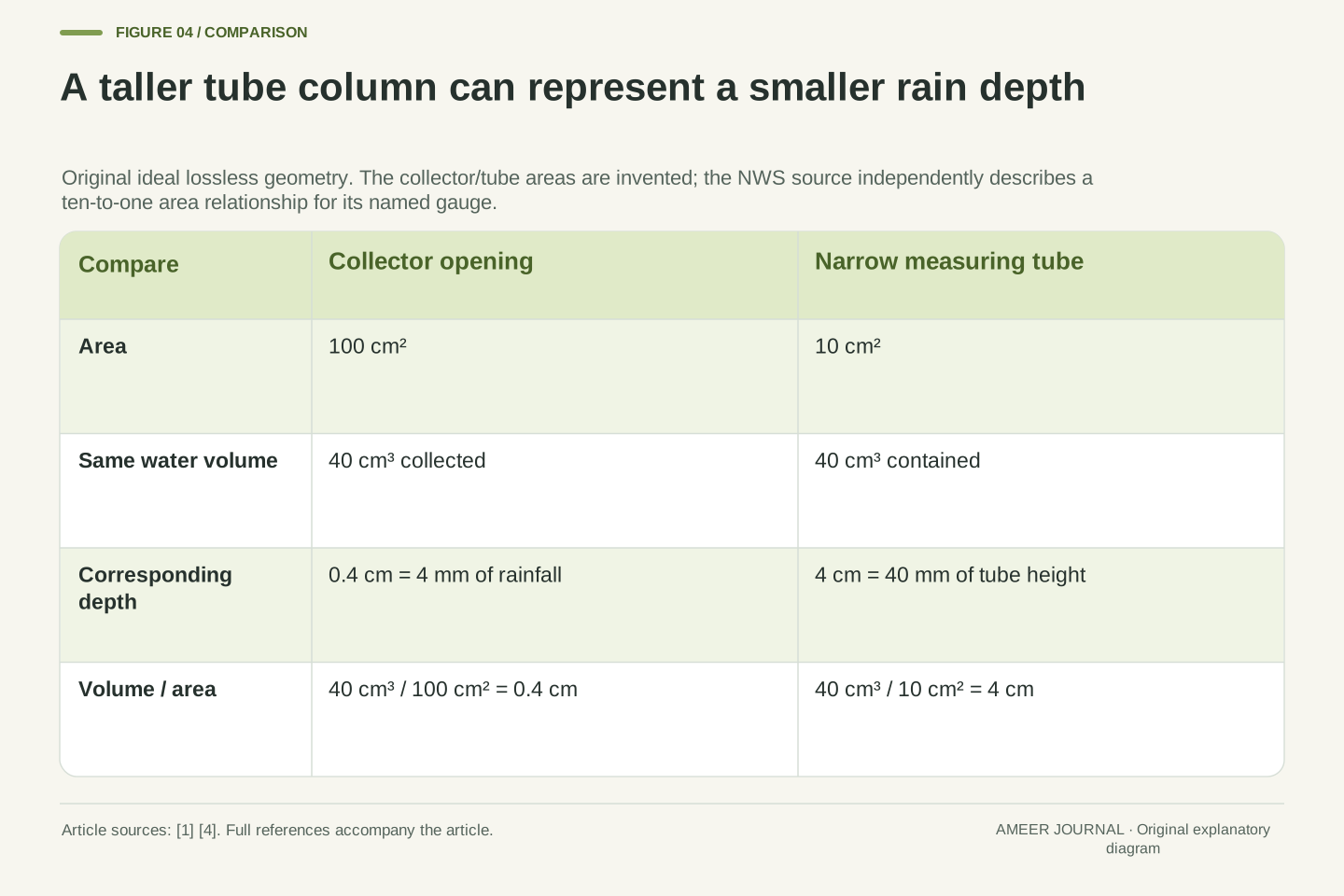
Some rain gauges guide water from a wide opening into a narrower measuring tube. The NWS description of its standard gauge says the opening area is ten times the tube area. The water column in that tube is therefore ten times as tall as the rainfall depth it represents [4]. The instrument's precipitation scale accounts for this change in shape.

Use our invented one-hundred-square-centimetre opening and a ten-square-centimetre tube. The forty cubic centimetres of collected water occupy a column four centimetres tall in the tube. That is forty millimetres of tube height, representing only four millimetres of rainfall over the wider opening. Forty and four describe different depths, so they do not contradict each other.

A label matters here. A scale marked in rainfall depth is not simply a ruler showing the water column's physical height. Our drawing explains the area ratio without asking anyone to make, open or measure a real instrument. It also does not claim that the invented areas are the dimensions of the NWS gauge.

Conservation of collected volume gives A_c H=A_t h, where A_c is collector area, A_t is measuring-tube cross-sectional area, H is rainfall depth and h is physical tube-water height. Thus h/H=A_c/A_t. The NWS source explicitly describes a ten-to-one area ratio for its named standard gauge [4]; this is not a property of every possible container.

The separate teaching geometry assigns A_c=100 cm² and A_t=10 cm². With V=40 cm³, h=V/A_t=4 cm=40 mm, while H=V/A_c=0.4 cm=4 mm. The factor of ten comes from area, not from a tenfold increase in incoming water. The dimensions are chosen for transparent arithmetic rather than copied from an eight-inch collector specification.

A calibrated precipitation scale can report H directly even though the observed water column has height h. Reading that scale and independently reading an ordinary length ruler would therefore require different interpretations. The calculation illustrates why a display's unit and calibration belong to the measurement record; it is not an instrument construction or calibration procedure.

Return to the card showing twelve millimetres over two hours. Divide twelve by two to get an average rate of six millimetres per hour. The words per hour are part of the answer. A number written as six millimetres would describe a depth, while six millimetres per hour describes a depth divided by time [2].

The same interval lasts one hundred and twenty minutes. Twelve divided by one hundred and twenty is 0.1 millimetres per minute. Multiplying that rate by sixty minutes per hour gives six millimetres per hour again. Changing the time unit changes the number used to write the rate; it does not change the rain card or its interval.

Think of the average as a steady rate that would produce the same total if it continued for the stated duration. That is a comparison we calculate, not a hidden observation of steadiness. The card has not supplied the moment when the rain started, the wettest minute, or what happened just after the two hours ended.

For positive elapsed duration Δt, define the interval-average rate as R̄=H/Δt. The quantity H is accumulated depth over exactly that same interval. This formalizes the accumulation-versus-rate distinction described by the Met Office [2]. It does not require the actual rate to have remained constant while the accumulation was collected.

The fixture gives R̄=12 mm/2 h=6 mm/h. In minute units, 12 mm/120 min=0.1 mm/min, and multiplication by 60 min/h recovers 6 mm/h. Dimensional consistency prevents confusing depth with depth per unit time. In particular, the number 12 must not be copied into a rate field merely because the original amount happened to be twelve millimetres.

For a specified piecewise-constant rate history, H is the sum of each segment's rate multiplied by its duration. The continuous counterpart is a time integral. An average is a summary of that integral, so many histories can share it. Neither an instantaneous value, a peak, the beginning of rain nor a continuation beyond the interval is determined by this one summary.

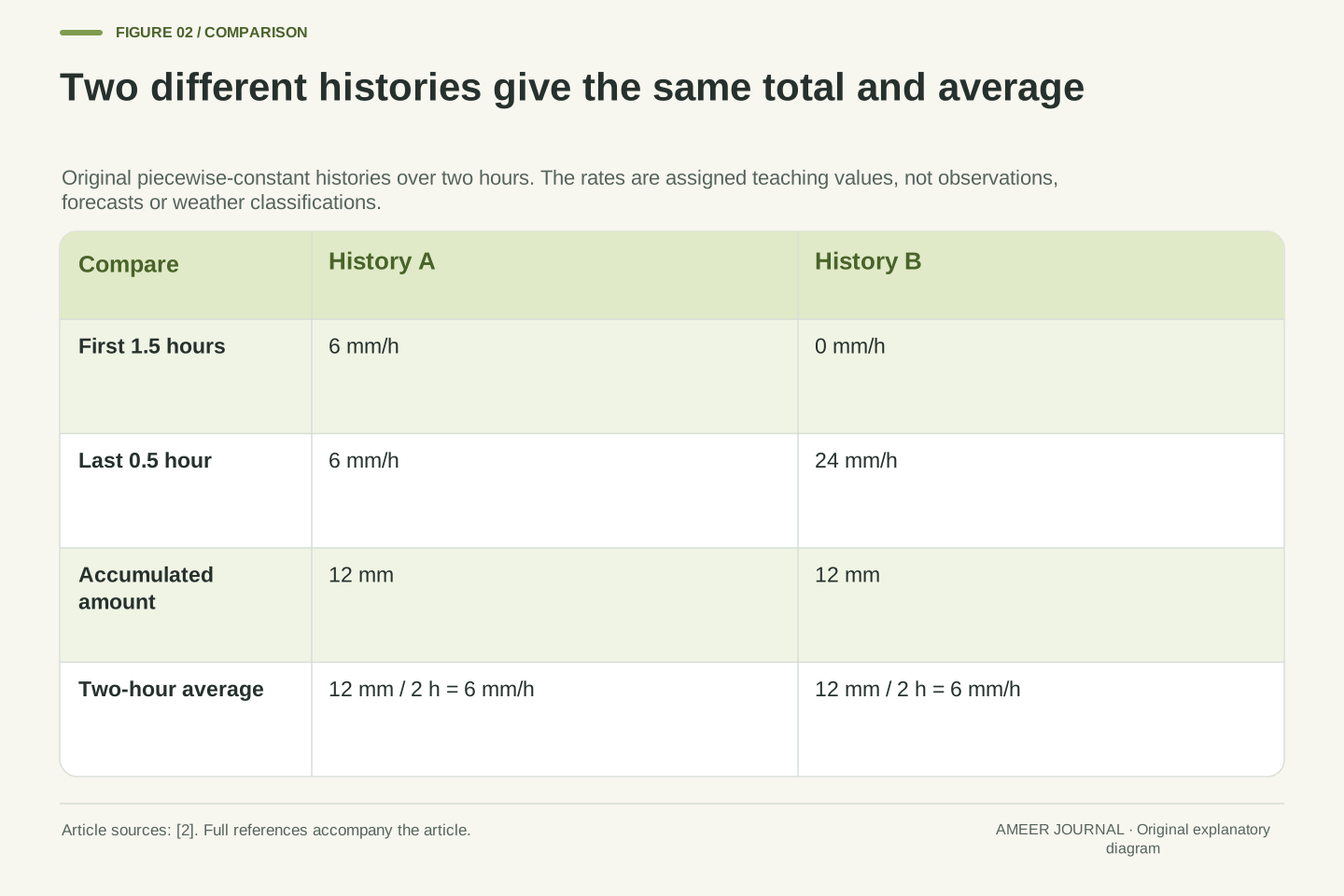
Paper history A is steady: six millimetres per hour for two hours. Its amount is six times two, which is twelve millimetres. Paper history B has no rain for the first hour and a half, followed by twenty-four millimetres per hour for the last half-hour. Its amount is zero plus twenty-four times one-half, also twelve millimetres.

The two histories therefore have the same total and the same two-hour average of six millimetres per hour. Yet their timing is very different. History A spreads the amount across the interval. History B puts all of it into the final half-hour. Both satisfy the information on the original card, so that card cannot choose between them.

The short rates were assigned to make the comparison checkable; they are not weather categories or claims about how real showers usually behave. If someone adds a new card saying when the rain fell, we can use that evidence. Until then, drawing a perfectly steady shower from an interval total would add information that was never recorded.

Define A by a constant 6 mm/h over 2 h. Its integral is 12 mm. Define B by 0 mm/h over 1.5 h and 24 mm/h over 0.5 h. Its integral is 0×1.5+24×0.5=12 mm. Both durations total 2 h, so both interval means equal 6 mm/h. These two explicit functions supply a counterexample to unique reconstruction from the total and duration.

The distinction is stronger than a rounding issue: the two exact totals agree while the rate functions differ over most of the interval. B also has a different maximum among its stipulated segment rates. A reported two-hour average therefore cannot be silently presented as the maximum rate or as the value at every observation time.

These are analytic histories, not sampled storms, probability models or an estimate of the frequency of intermittent rainfall. Additional timed observations can rule out one or both candidates, but the original two-hour record cannot. The accumulation/rate distinction is source-supported [2]; the exact pair and its non-uniqueness demonstration are original calculations under the stated piecewise-constant assumptions.

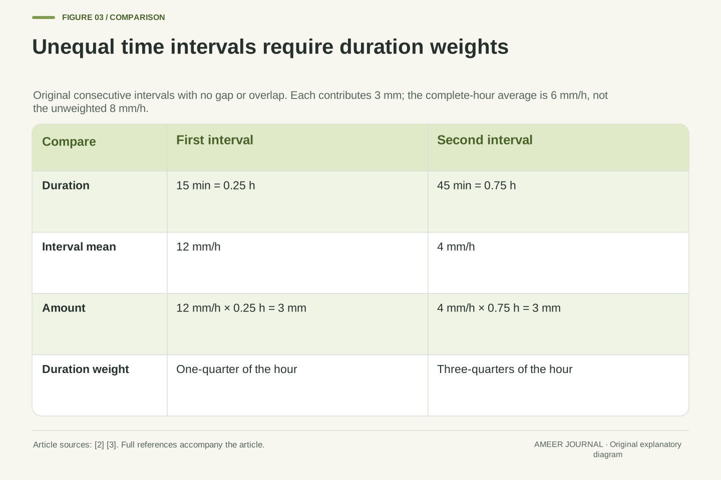
Now imagine two neighboring time cards. The first covers fifteen minutes at an average of twelve millimetres per hour. The second covers forty-five minutes at an average of four millimetres per hour. Fifteen minutes is one-quarter of an hour, so the first card contributes three millimetres. Forty-five minutes is three-quarters of an hour, so the second also contributes three.

Together, the cards cover one complete hour and contain six millimetres. The combined average is therefore six millimetres per hour. Simply averaging twelve and four gives eight, which is wrong for this whole-hour question. The slower rate lasted three times as long, so it must have three times as much influence on the time average.

The reliable route is to recover each interval's amount, add those amounts, then divide by the total duration. This assumes the cards cover consecutive periods without a gap or overlap. If one minute were counted twice or an interval were missing, the same addition would no longer describe one complete, nonoverlapping hour.

For disjoint intervals with durations Δt_i and interval means R̄_i, the combined mean is Σ(R̄_iΔt_i)/ΣΔt_i. It is a duration-weighted mean. This follows from adding the accumulated amounts over the same observation boundary, consistent with the agency descriptions of interval accumulations [2][3]. No assumption of equal interval lengths should be introduced during aggregation.

The original pair is (Δt_1,R̄_1)=(1/4 h,12 mm/h) and (Δt_2,R̄_2)=(3/4 h,4 mm/h). Each contributes 3 mm, so the pooled result is (3+3) mm/(1/4+3/4) h=6 mm/h. The unweighted arithmetic mean (12+4)/2=8 mm/h assigns equal weight to unequal durations and answers a different numerical question.

The pooled calculation needs compatible units, a common quantity definition and a complete partition of the target interval. Overlapping windows double-count some accumulation; gaps leave part of the desired total unknown. These conditions concern the records being combined, not whether either individual average was calculated correctly. A correct local average does not automatically make an arbitrary collection of windows additive.

A tipping-bucket rain gauge fills a small bucket until it tips, then another bucket takes over. A recorder counts these events. The Met Office and Australian Bureau of Meteorology describe instruments whose tips correspond to a nominal increment of 0.2 millimetres [1][3]. That number belongs to the described instruments; a different gauge needs its own specification.

Our paper recorder also uses 0.2 millimetres per tip. Five recorded tips therefore earn five increments, totaling one millimetre. If those events fall within a ten-minute reporting window, the nominal reported average is six millimetres per hour: one millimetre divided by one-sixth of an hour. We have calculated a rate from the event record.

Keep the word recorded in the sentence. The bucket may contain an unfinished increment at the beginning or end of a window. Also, actual instruments can lose some water while collecting or tipping [4]. Counting complete increments is useful, but it does not make every possible window an exact record of all physical water that arrived.

A tipping-bucket mechanism converts accumulated input into discrete events when a fill threshold is reached. The named instrument descriptions use a nominal rainfall-depth increment of 0.2 mm per tip [1][3], while the Met Office explains how counts and timing support accumulation and rate reporting [2]. The increment is a calibration parameter, not a universal constant of rainfall.

For the fictional recorder, set q=0.2 mm per event. A count n=5 gives nominal credited depth nq=1 mm. Over Δt=10 min=1/6 h, the nominal reported average is nq/Δt=6 mm/h. This computation specifies a count-based reporting convention; it is not a reconstruction of instantaneous input between events.

Finite increments and physical measurement limitations remain separate. Even an ideal lossless counter can carry an incomplete increment across a window boundary. Real instruments can additionally have collection or tipping losses, as the NWS discussion explains [4]. No historical error percentage or correction algorithm from that source is transferred to our fictional recorder, and no actual gauge performance has been measured.

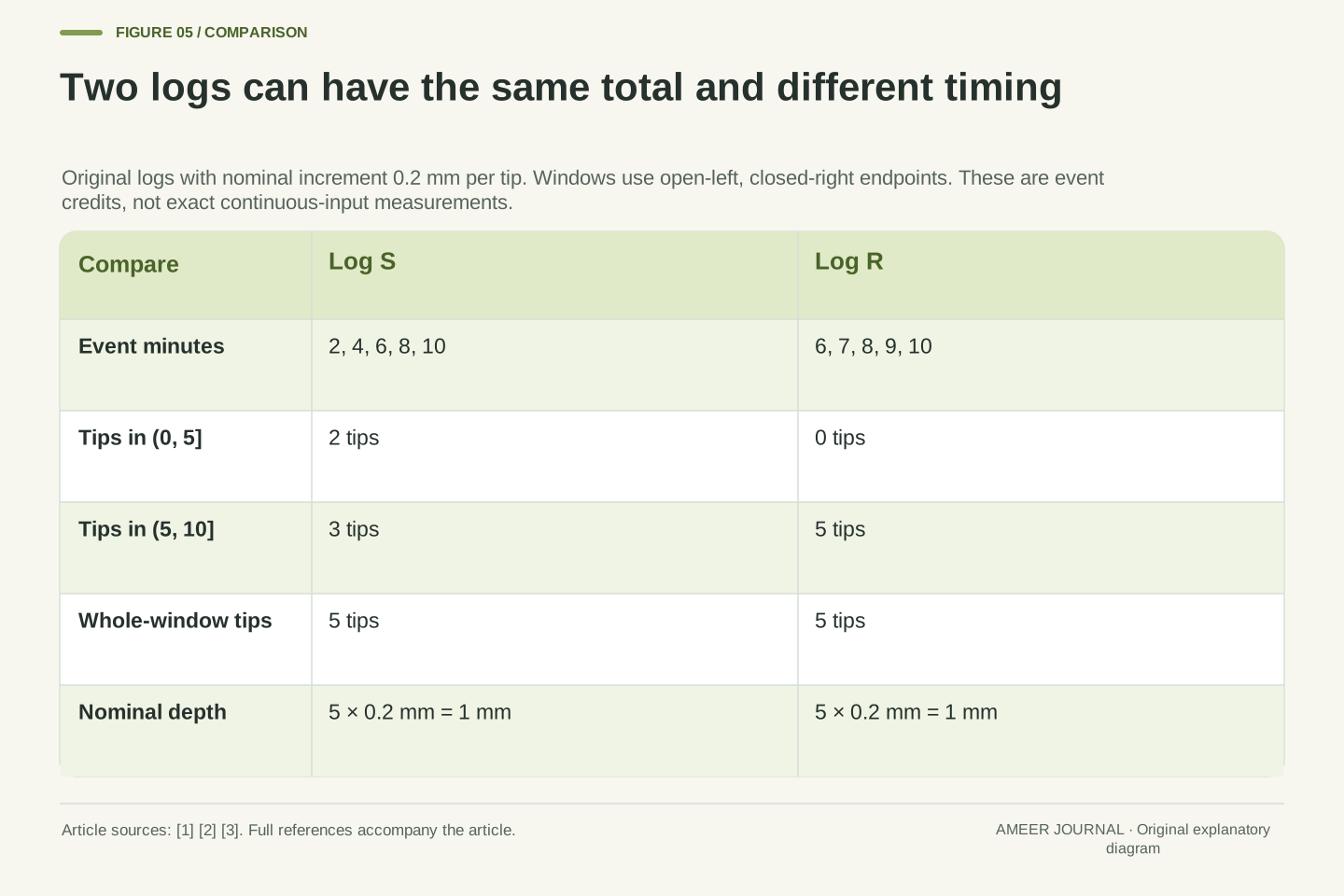
Paper log S records tips at minutes two, four, six, eight and ten. Paper log R records them at minutes six, seven, eight, nine and ten. Each log contains five events in ten minutes. If we save only the total count, both logs become the same one-millimetre nominal report, even though their event times are different.

Split each log into the first five minutes and the last five. S has two events in the first part and three in the second. R has none in the first part and five in the second. The detailed event lists preserve this distinction. It disappears when the entire ten minutes are reduced to one count.

For S, the nominal half-window amounts are 0.4 and 0.6 millimetres; for R, they are zero and one. These are credits attached to recorded events. A zero event count does not yet prove that no water entered during those minutes. The next example explains why a bucket can be filling before it has enough water to make a new tip.

Define S={2,4,6,8,10} and R={6,7,8,9,10}, with event times in minutes from a declared origin. Count events in open-left, closed-right windows (0,5] and (5,10], so the windows partition (0,10] without counting a boundary event twice. S produces counts (2,3); R produces (0,5). Both complete-window counts equal five.

With q=0.2 mm, the nominal half-window depths are (0.4,0.6) mm for S and (0,1) mm for R. Each half lasts 1/12 h, giving nominal reported rates (4.8,7.2) mm/h and (0,12) mm/h respectively. Both full-window reports remain 1 mm over 1/6 h, or 6 mm/h. These are exact event-credit calculations.

Timed events contain more information than a total event count, consistent with the documented tipping-bucket use [2][3]. They still do not specify a unique continuous inflow within each fill interval. In particular, a window without a tip can contain an unfinished increment. The distinction between nominal credits and physical input prevents interpreting R's first zero count as a demonstrated dry interval.

Imagine an ideal paper bucket that tips at 0.2 millimetres of equivalent collected rain. It begins a short interval with 0.04 millimetres already inside and ends with 0.13 millimetres. It has gained 0.09 millimetres, but it has not reached the tipping mark. No event is recorded even though water has arrived.

This example assumes perfect collection, no loss and no emptying. It shows a limitation that can exist even before we discuss a real instrument's errors. A tip is evidence that an increment has finished. The absence of a tip over a short period is not the same statement as a complete measurement of zero incoming water.

An unfinished amount can also affect a period with several tips. Five completed 0.2-millimetre increments give one millimetre of event credits. If the unfinished amount grows from 0.05 to 0.15 millimetres during that period, the ideal incoming amount is 1.1 millimetres. The extra 0.1 remains inside at the end instead of appearing in a completed increment.

Model an ideal lossless threshold counter with increment q, no reset and equivalent-depth remainders r_start and r_end satisfying 0≤r<q. Conservation gives incoming depth H=nq+r_end−r_start. The source-described filling-and-tipping mechanism motivates this bookkeeping [2][3]; the equation and chosen endpoint states are an original idealization, not a firmware or accuracy specification.

With q=0.2 mm, n=0, r_start=0.04 mm and r_end=0.13 mm, H=0.09 mm. Both endpoint remainders stay below the threshold, so zero events coexist with positive input. With n=5, r_start=0.05 mm and r_end=0.15 mm, H=1.1 mm while nq=1 mm. Every assigned endpoint is within the model's permitted range.

Nominal event credits equal physical interval input in this idealization when the endpoint remainders match. Otherwise their difference is r_end−r_start, whose magnitude is less than q. Real evaporation, collection losses or tipping behavior introduce additional terms rather than invalidating the distinction [4]. We do not estimate those terms, infer actual dry weather from a zero count or claim the ideal bound describes a real instrument's total error.

A record called daily rain still needs its observation times. The Met Office's storage-gauge description uses a morning reading, while the Australian Bureau describes a nominal morning observation and sometimes longer accumulated periods [1][3]. These examples show why a daily label should not automatically be read as midnight to midnight everywhere.

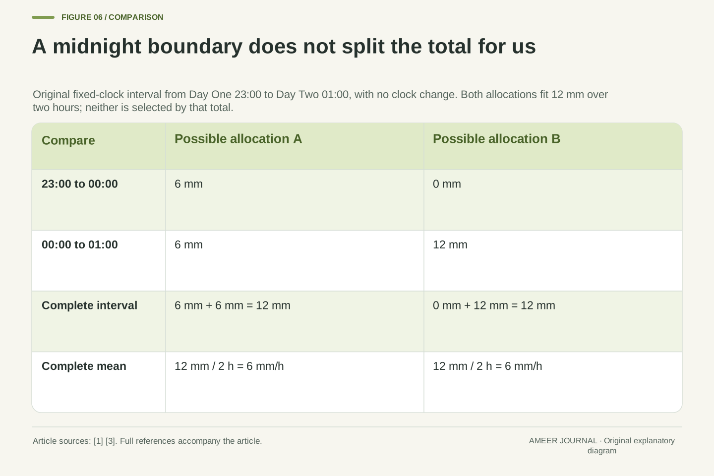
Our next card runs from eleven at night on Day One to one in the morning on Day Two. Using a fixed clock with no time change, that is two hours. The card reports twelve millimetres. Six could belong to the hour before midnight and six to the hour after it. Or zero could belong to the first hour and twelve to the second. Both fit the same whole-interval total.

The date change does not divide the rain for us. To assign an amount to each side of midnight, we need a record that resolves those parts or an explicitly stated estimate. Splitting the total in half is one possible assumption, not a fact established by the original card.

Observation-period boundaries are part of the datum. The Met Office describes a 0900 UTC storage-gauge reading, while the Bureau describes nominal 9am local observations and occasional 48- or 72-hour accumulations [1][3]. These are attributed descriptions of observing practice, not a universal claim about every current station or an instruction to collect data.

The original midnight example uses one fixed reference clock with no daylight-saving or timezone transition. From Day One 23:00 to Day Two 01:00, Δt=2 h. Given H=12 mm, the hour-pair assignments (6,6) mm and (0,12) mm are both compatible with the record. The resulting full-interval mean is 6 mm/h in either case.

The total therefore cannot determine a calendar-day allocation at midnight. A time-resolved record or an explicit imputation model would be additional information, and an imputed split must remain distinguishable from an observation. Similarly, assigning a daily record to its ending date does not by itself change the physical start of its accumulation interval. Preserve both timestamps and their time reference.

Suppose one interval on a weather sheet is blank. The blank might mean the reading is unavailable; it is not a measured zero. If an earlier card is missing and a later card reports two millimetres, the later value alone cannot tell us the total for both periods. Adding an invented zero would make the sheet look complete without adding evidence.

A real gauge also samples a particular opening at a particular place. Its surroundings and collection behavior can affect what it catches. The agency sources discuss collector area, wind effects and differences between gauge designs [1][3][4]. Those details explain why a neat number still needs a description of how it was obtained.

Our paper records avoid those measurement complications by declaring the quantities exactly. A real local reading would not, by itself, prove the same amount fell across a whole town, reveal every minute of a shower, or show whether a road will flood. Each further question needs information at its own place, time and measurement boundary.

Missing data and measured zero are distinct record states. A zero can be an explicitly defined amount or event count; a missing interval supplies neither. Summing only the available amounts does not establish a total over a longer interval containing gaps. Filling a gap with zero is an assumption or reporting policy, not a consequence of the missing record.

Spatial sampling and instrument response impose separate limits. The collector defines a sampling area [1], and the Bureau and NWS describe influences such as aperture, wind and differences in catch [3][4]. Those sources justify retaining method and context; they do not supply a universal correction for our nonexistent instrument or an uncertainty distribution for the invented numbers.

Our exact identities hold within the stated geometric and temporal models. They do not demonstrate city-wide uniform rainfall, gauge calibration quality, a storm's future intensity or flood risk. A complete interpretation identifies which value is an accumulated depth, a nominal event-credit quantity, an interval mean or a missing observation before combining it with another record. These distinctions prevent precision in arithmetic from being mistaken for completeness of evidence.

With an adult, choose the twelve-millimetre card, the unequal-interval pair and the two tip logs. Point to the amount and the start and end of each interval. Ask which answer comes from the given record and which would need extra information. You can discuss the answers aloud; there is no score, timer, account or request to send your work.

For the first card, say: twelve millimetres over two hours gives an average of six millimetres per hour, but it does not tell us the within-interval pattern. For the second, say: three millimetres plus three millimetres over one complete hour also gives six millimetres per hour. The two average rates happen to match, although the records describe different situations.

For the tip logs, say: both have five events in ten minutes, while their event times differ. The first five minutes of R contain no recorded tip, which is different from proving that no water arrived. A useful weather sentence keeps the amount, unit, interval and kind of record together. The unanswered question stays visible instead of being quietly replaced with a guess.

The final exercise asks an adult and child to interpret three existing fictional records, not collect new measurements. For each statement, identify the quantity, unit, observation interval and available temporal detail. The distinction between accumulation and rate comes from the documented measurement concepts [2]; the assigned numbers make each inference independently reproducible.

The twelve-millimetre record supports H=12 mm, Δt=2 h and R̄=6 mm/h, with a non-unique rate history. The unequal-duration pair supports H_1=H_2=3 mm and a pooled 6 mm/h rather than the unweighted 8 mm/h. The two event schedules support identical ten-minute nominal totals but distinct half-window event-credit patterns. None of these statements requires an actual weather experiment.

Finally distinguish a fact supplied by a record from a model chosen to interpret it. The ideal remainder equation explains why complete increments can miss partial input at a boundary; real measurement quality would require additional evidence. The private paper lesson succeeds when the reader can state a justified average and also name the time structure that remains unknown. No child data, location, photograph, weather report or online response is requested.