What you’ll take away
- A water-permeable cell can have zero mean net water transfer while retaining solute, when the relevant total water potentials match.
- Compare the total solute and pressure contributions under the stated conditions; a concentration comparison alone omits pressure.
- The finite-volume example uses an invented pressure rule and ideal dilute solute behavior. Its balance at 1.20 times the reference volume is a calculation, not a plant measurement.
- Zero mean net transfer does not mean motionless molecules. An unchanged amount also needs its boundary conditions explained.
A dissolved substance does not keep water entering forever
Picture a tiny plant cell with dissolved material inside. Must water outside keep entering until all that material disappears? It need not. A cell can reach a balance at which its water amount has no continuing upward trend even though dissolved substances remain. The missing clue is pressure. Water entering a plant cell can increase the pressure supported by its surrounding cell wall. That pressure can balance the effect of dissolved material on water movement. [1][2]
We will investigate this with invented drawings and numbers. A solute is a substance dissolved in a liquid; in our examples, water can cross the cell's membrane while the named solute stays inside. Read with a grown-up and use this screen or an uncut sheet of paper. First we will compare three separate cell cards. Then we will let the liquid volume change in an imaginary cell with a clearly stated rule. These are reasoning puzzles, not observations of a plant or instructions for an experiment.
A plant cell can reach equilibrium with respect to passive water transfer while retaining an unequal solute concentration across its membrane. Hydrostatic pressure can counterbalance the solute contribution to water potential. OpenStax explicitly describes pressure balancing osmosis, and its plant-transport chapter separates the components of total water potential. [1][2] Thus, the presence of an impermeant solute does not by itself establish that net water influx must continue indefinitely.
The examples below use a water-permeable, solute-impermeable boundary, a common temperature and height reference, and no active solute transport. They first compare independent stipulated states, then introduce a separate one-compartment model whose solution volume can vary. Every numerical value and the model's pressure law is hypothetical. The goal is to identify an equilibrium condition and its limits, without presenting a cell measurement, species prediction or physical procedure. The optional activity is adult-supported screen or uncut-paper reasoning; the technical mode develops the same account with explicit algebra.
Give the membrane and the wall different jobs
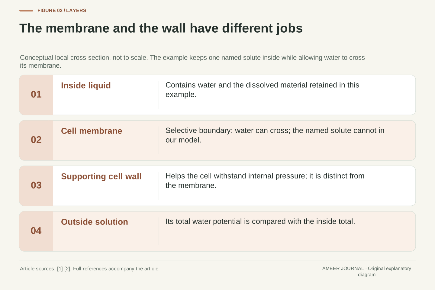
A plant cell has a thin membrane and a supporting cell wall outside it. The membrane is selective: substances do not all cross it in the same way. The wall helps the cell withstand pressure from its contents. These are different jobs, so draw and label them separately. A membrane that water can cross is not the same thing as an open hole that lets every dissolved substance escape. Our rule that the chosen solute cannot cross is a rule for the puzzle. [1][2]
The movement of water across a selectively permeable membrane is called osmosis. Membrane proteins can provide pathways for water, while the membrane limits the passage of other substances. [2] In our drawing, count two different things: the dissolved material kept inside, and the water that may enter or leave. If water enters, the first count need not increase with it. If we changed the rules so that the solute could also move, we would need a new account of both quantities before using the later calculations.
Selective permeability concerns the plasma membrane, whereas mechanical support from the surrounding cell wall permits positive turgor pressure. Water pathways can include aquaporin proteins; permeability to a particular solute is a separate property. [1][2] The illustrations are local conceptual cross-sections, not scaled anatomical drawings. They distinguish the intracellular solution, membrane, supporting wall and exterior solution without asserting that all real solutes are permanently confined by every plant membrane.
For the mathematical construction, the amount of the selected dissolved particles is fixed, and the compartment exchanges water only. This is stronger than saying merely that a real membrane is selective. It supplies the conservation assumption later used to relate concentration to volume. A model allowing solute uptake, leakage or chemical production would require an additional solute balance. The wall's mechanical role also does not make it an active valve: pressure can oppose further net influx while the membrane remains permeable to water. [1][2]
A water-potential number is not a water counter
Biologists use a quantity called water potential to compare the tendency for water to move between places. It is written with the Greek symbol Ψ. The reference is pure water under stated conditions, and the values use pressure units, often megapascals, written MPa. [1] You do not need to handle pressure equipment to read our numbers. Think of them as labels to compare under the same rules. A value of zero is the chosen reference; it does not mean that no water is present.
Some labels have a minus sign. On an ordinary number line, −0.10 is higher than −0.30, which is higher than −0.60. The minus sign does not describe a negative amount of water. Nor does a larger drawing automatically have a higher water potential. Two differently sized portions can have the same concentration and pressure. Our question is which side has the higher comparison value, not which side contains more liquid. Mixing those questions would make a large outside supply look like a reason for endless filling.
Water potential Ψ is expressed relative to a specified pure-water reference, using pressure units rather than units of volume or an absolute total-energy inventory. OpenStax uses MPa and distinguishes solute, pressure, gravitational and matric contributions. [1] One MPa equals one million pascals. The relevant comparison is a difference between consistently referenced states; simply knowing the amount of water in each compartment does not supply that difference.
Signed ordering must be retained: −0.10 MPa > −0.30 MPa > −0.60 MPa. A less negative value is the higher potential. As a logical example, scaling both solution volume and solute amount by the same factor preserves concentration; if the other modeled conditions are also unchanged, it need not change Ψ. This distinguishes an intensive state description from an inventory. The zero reference likewise does not assert zero water, zero molecular motion or zero absolute energy. These distinctions matter before applying a direction rule to the numerical cards.
Add the effects before comparing the two sides
For our simple cell puzzle, the total has two entries. One is the dissolved-material part, called solute potential. In the mixtures used here it is negative. The other is the pressure part: positive pressure contributes a positive number. Add them to obtain the total water potential. A large negative entry can therefore be balanced partly or completely by a positive entry. The plant-transport and university teaching sources describe this combination of solute and pressure contributions. [1][4]
The full account can also include height and interactions with solid surfaces. [1] Our imaginary inside and outside use the same temperature and reference height, and we set the omitted surface contribution to zero. Those are simplifying choices. Once the conditions are fixed, compare the two totals. For a passive boundary water can cross, the mean net tendency is from higher total water potential to lower total water potential. [1] Comparing only the dissolved-material entries would leave pressure out of the question we are trying to answer.
The retained native equation is Ψtotal = Ψs + Ψp + Ψg + Ψm, with solute, pressure, gravitational and matric terms. [1] Here the two sides share a height reference and the omitted contributions are stipulated to be zero, giving Ψ = Ψs + Ψp. Colorado State University's teaching account also uses an explicitly simplified osmotic-plus-turgor sum. [4] This reduction is an assumption of the construction, not a claim that gravity or surface interactions never matter in plants.
For an ideal dilute solution, the solute relation can be written Ψs = −iCRT, where C is solute molar concentration, i accounts for dissolved particle number, R is the gas constant and T is absolute temperature, with consistent units. [1] Positive hydrostatic pressure raises Ψp relative to the chosen pressure reference. Under our passive, water-permeable, impermeant-solute conditions, the total difference determines the direction of mean net transfer. [1] Neither the most negative component alone nor a comparison of liquid amounts can replace that sum.
Read three separate cell cards
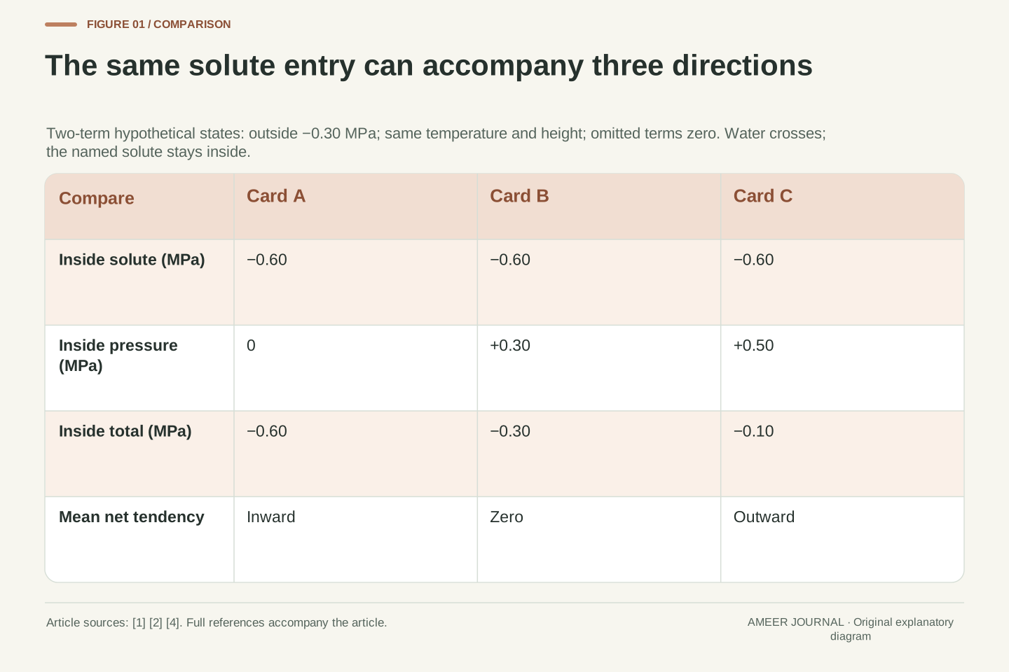
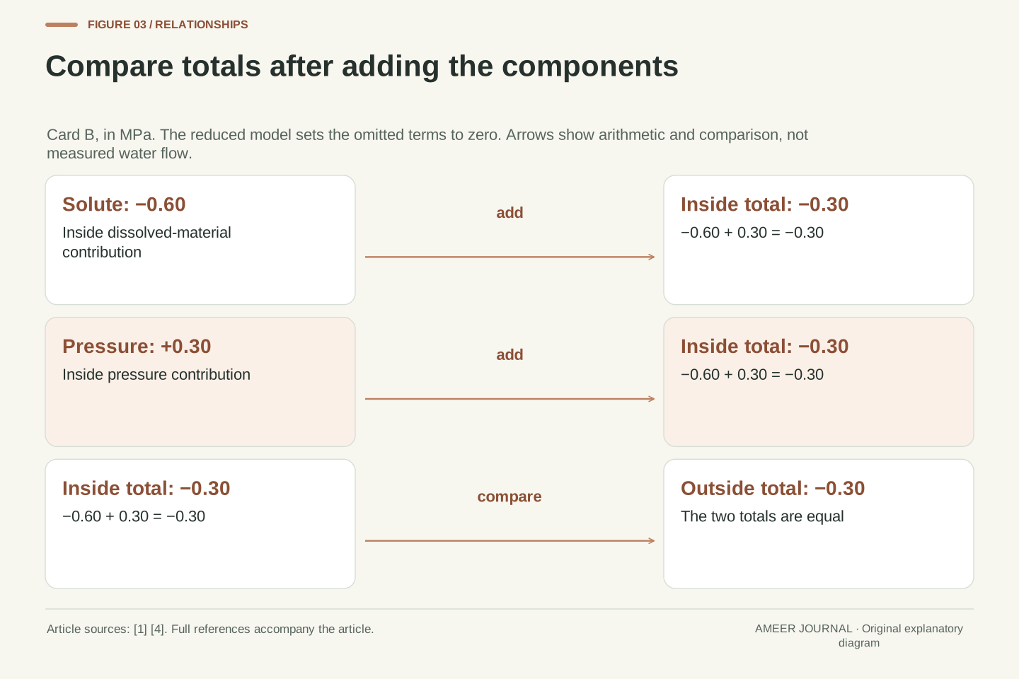
Put −0.30 MPa on the outside of each card. Give every inside the same dissolved-material entry, −0.60 MPa. On card A, the pressure entry is zero, so the inside total is −0.60 MPa. The outside total, −0.30, is higher. The predicted mean net tendency is inward. On card B, the inside pressure entry is +0.30 MPa. Adding −0.60 and +0.30 gives −0.30 MPa, exactly the outside total. This card has no mean net transfer driven by a total-potential difference. [1]
Card C has an inside pressure entry of +0.50 MPa. Its total is −0.60 + 0.50 = −0.10 MPa. Now the inside total is higher than the outside's −0.30, so the mean net tendency is outward. The same dissolved-material entry appears on all three cards, yet the answers differ. These are three separate invented states, not a film of one cell filling. We have assigned different pressure entries without claiming that a real cell passes through them while its concentration stays fixed.
Let Ψout = −0.30 MPa and stipulate Ψs,in = −0.60 MPa for three independent records. Set Ψp,in to 0, +0.30 and +0.50 MPa. The corresponding inside totals are −0.60, −0.30 and −0.10 MPa. Defining D = Ψout − Ψin gives +0.30, 0 and −0.20 MPa. With the stated passive permeability conditions, the signs indicate inward, zero mean net, and outward transfer tendencies respectively. [1] No flow-rate coefficient or elapsed time has been assigned.
The construction is a counterexample to choosing direction from the solute term alone. It holds that term fixed while changing the pressure contribution across independent records. It does not prescribe a sequence of attainable states for one biological cell or demonstrate that its solute concentration would remain fixed during swelling. In particular, pressure is an assigned state variable here, not a measured consequence of a specified wall law. The later volume model supplies such a law separately and uses different starting values.
Equal totals do not require equal mixtures
Look more closely at balanced card B. We can make its outside total from a dissolved-material entry of −0.30 MPa and a pressure entry of zero. Inside, the entries are −0.60 and +0.30 MPa. The totals match even though the entries do not. The inside still contains its dissolved material, and its pressure is still positive. Nothing in the addition says that the solute had to escape or that the inside became pure water. Pressure has supplied the balancing contribution. [1][2][4]
This is why the sentence “water moves toward the side with more dissolved material” needs conditions. It leaves out what pressure is doing. In our balanced example, different dissolved-material contributions coexist with equal total water potentials. If the outside total later changed, we would compare again; an earlier balance would not settle the new question. Also, matching totals does not tell us that the two sides have equal volumes. The information on the card concerns the balance, not the size of the containers.
For card B, choose exterior components Ψs,out = −0.30 MPa and Ψp,out = 0. The inside-minus-outside differences are then ΔΨs = −0.30 MPa and ΔΨp = +0.30 MPa. Their sum is zero. Thus, Ψin = Ψout does not require Ψs,in = Ψs,out or Ψp,in = Ψp,out. Under the same ideal-solute and temperature assumptions, unequal solute contributions can correspond to unequal concentrations at water equilibrium. The pressure-balance qualification is explicit in the osmosis source. [2]
This is an equilibrium condition for water exchange across the stated boundary, not a requirement that impermeant solutes equilibrate by crossing it. The additive account permits differences in components while their totals agree. [1][4] It also does not identify a compartment volume without information about solute amount and pressure mechanics. Changing the external potential would generally change the equality to be satisfied. Consequently, a balanced state should be described together with its boundary and conditions, rather than treated as a permanent property of a cell.
Let concentration and pressure change together
Now start a separate imaginary model. The outside is maintained as pure water with total potential zero. The inside keeps a fixed amount of dissolved material. Call its starting liquid volume one unit. If the volume later becomes 1.20 units, the same dissolved material is spread through more liquid. Its concentration becomes 1 divided by 1.20, or five-sixths of its original concentration. The amount stayed fixed while the concentration fell. This is the distinction used in the ideal dilute solute relation. [1]
We also invent a simple pressure rule for the model's supporting wall: each increase in relative volume adds the same numerical increase in MPa to its pressure entry. Thus, relative volume 1.00 gives zero pressure, while 1.20 gives +0.20 MPa. The rule is chosen for this puzzle; it is not a measured rule for plant walls. Together, dilution and the increasing pressure entry change the total as water enters. We can now ask where the model balances, instead of merely assigning an already balanced card.
Introduce a new model with fixed dissolved particle amount, fixed temperature and a maintained exterior reservoir at Ψout = 0 MPa. Write x = V/V0, where V is the modeled intracellular solution volume and V0 its reference volume. The domain is x ≥ 1. Since C = n/V with n fixed, C/C0 = 1/x. The ideal dilute relation therefore permits the assigned solute law Ψs(x) = −0.24/x MPa. [1] The coefficient is an original teaching choice, not a cytoplasmic measurement.
Stipulate the separate pressure law Ψp(x) = (x − 1) MPa. This linear dependence is an invented constitutive assumption; the sources support pressure's role, not this particular stiffness or volume range. [1] At x = 1.20, concentration is 5/6 of its initial value, a decrease of 1/6, while solution volume has increased by 20 percent. The different percentages have different denominators. V is the single modeled solution compartment's volume, not a whole-plant mass, an anatomical inventory of organelles or a direct count of water molecules.
Find a balance at a finite volume
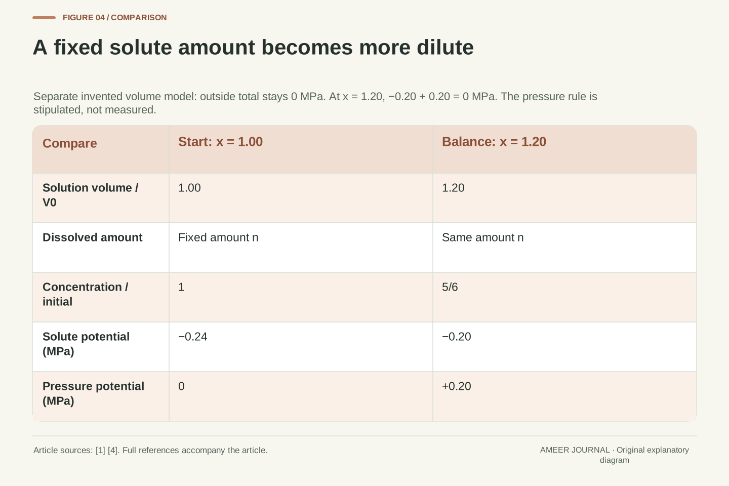
At relative volume 1.00, the model's dissolved-material part is −0.24 MPa and its pressure part is zero. Its total is therefore below the outside's zero, giving an inward tendency. Now check relative volume 1.20. The dissolved-material entry is −0.24 divided by 1.20, or −0.20 MPa. The pressure rule gives +0.20 MPa. Add them: −0.20 + 0.20 = 0. The inside total matches the maintained outside total at a finite volume. That is the balance condition from the sources. [1][4]
The model did not need to wash its solute away. It still has the same dissolved amount, spread through 1.20 times the starting solution volume. The pressure entry remains positive. Nor did the membrane have to turn into a closed door. Within the model, the two contributions now sum to the exterior value. You can verify the answer just by substitution and addition. The twenty-percent increase describes this invented solution volume; it is not a promised change in a real cell, its water mass or an entire plant.
Equilibrium requires Ψin(x) = Ψout, hence −0.24/x + x − 1 = 0 when the potentials are expressed in MPa. Multiplying by positive x gives x² − x − 0.24 = 0. Its discriminant is 1.96, whose square root is 1.4, so the roots are 1.20 and −0.20. Only 1.20 lies in the stated domain x ≥ 1. Substitution yields Ψs = −0.20 MPa, Ψp = +0.20 MPa and Ψin = 0, matching the maintained reservoir. [1][4]
The negative algebraic root is not another cell state; it violates the volume definition. The accepted root preserves the fixed solute amount and leaves a nonzero concentration, 5/6 of its initial value. This exact calculation demonstrates that the chosen combination of ideal dilution and increasing pressure admits a finite balance. It does not establish the same expansion for any biological wall, determine how quickly the state is approached, or prove that a measured unchanged volume must arise from this mechanism. Those would require additional evidence beyond the equilibrium equation.
Check which way the model tends on either side
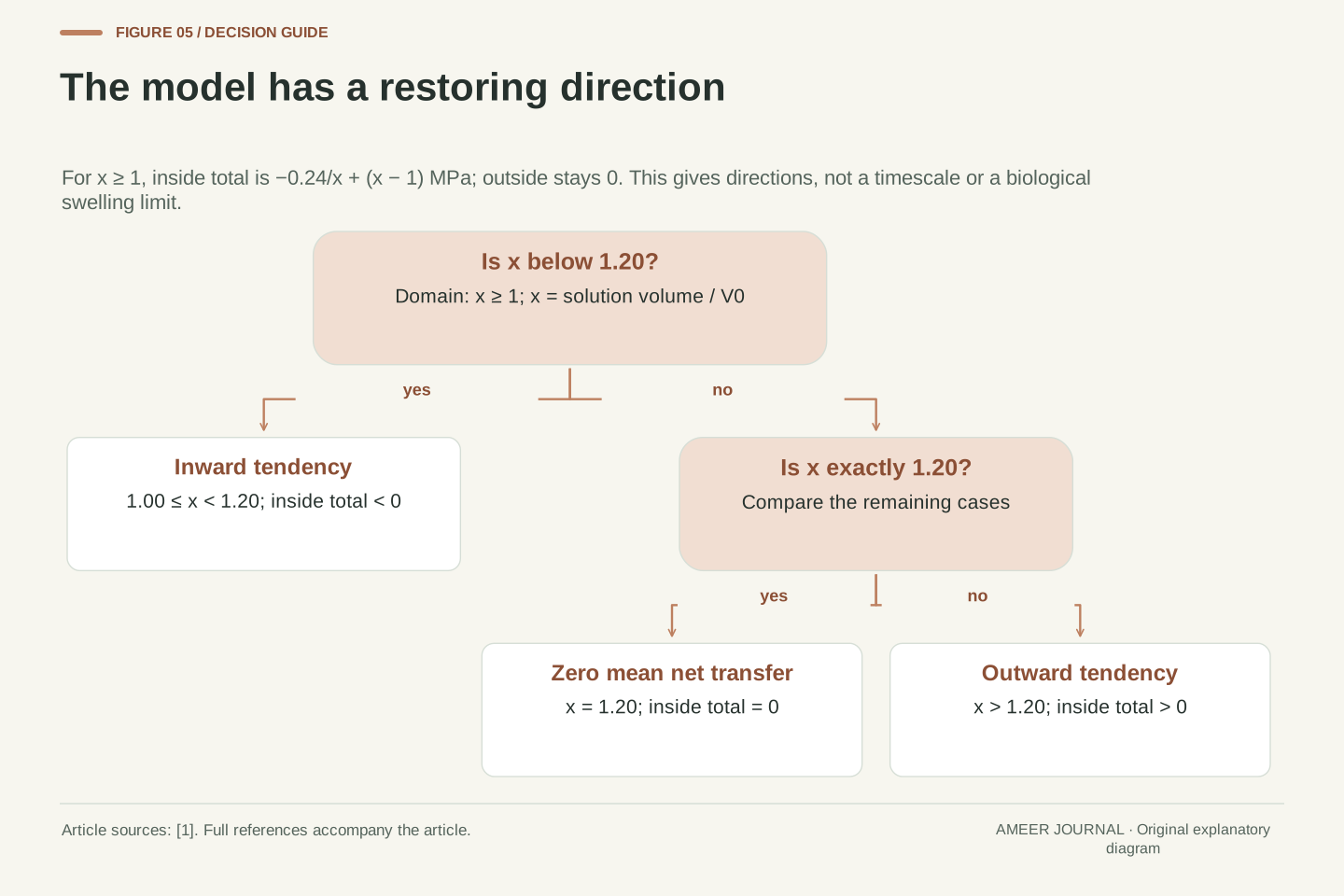
What if the model were at relative volume 1.25 instead? Its dissolved-material part would be −0.192 MPa and its pressure part +0.25 MPa. Their sum is +0.058 MPa, higher than the exterior's zero. Under our rules, the mean net tendency would be outward. At the starting volume 1.00, the opposite tendency was inward. The two checks lie on opposite sides of the balance at 1.20, and both point back toward it. These are calculated states, not readings from an experiment.
There is a reason the pattern holds between those examples. As the model's volume increases, its dissolved-material entry becomes less negative and its pressure entry increases. Both changes raise the total. Below the balance the total is lower than outside; above it, higher. The high-to-low rule therefore supplies a restoring tendency within this model. [1] It gives a direction, not a clock. We have supplied no information about how much water crosses in a second, how quickly a real cell responds or how much swelling it can tolerate.
The sign can be checked without relying only on sampled states. Factor the dimensionless numerical expression as f(x) = −0.24/x + x − 1 = (x − 6/5)(x + 1/5)/x. In the model domain x ≥ 1, the second factor and denominator are positive. Thus f is negative below 6/5, zero at 6/5 and positive above it. Combining this sign with Ψout = 0 and the passive transfer direction gives a restoring tendency toward the equilibrium. [1]
For exact checks, x = 1.10 gives Ψin = −13/110 MPa, while x = 1.25 gives Ψin = 29/500 MPa, or +0.058 MPa. More generally, for y > x > 0, f(y) − f(x) = (y − x)(1 + 0.24/(xy)) > 0. These are original algebraic properties of the stipulated model. No kinetic law, permeability value or biological pressure-volume curve was supplied. Therefore the calculation establishes the directional feedback and unique domain-valid balance, not a relaxation time, a safe swelling range or a measured response trajectory.
Balanced water has not stopped moving
The word net is important. It compares movement in one direction with movement in the other. At a balanced water-permeable boundary, zero mean net transfer does not mean every water molecule has stopped. Molecules continue their thermal motion, and water can still cross in both directions. The sources call a balance with continuing molecular movement dynamic equilibrium. [2] We are describing no continuing average gain on one side, not a promise that exactly matching numbers cross during every tiny instant.
A still-looking drawing also cannot tell us everything about its boundary. Imagine a different puzzle in which water cannot cross at all. The inside amount could stay unchanged even if the two potential values differed. That would be a blocked route, not the water-equilibrium explanation used above. So first ask whether the stated boundary allows water through. Then ask whether the total potentials match. The same simple observation, an unchanged amount, does not by itself establish which of those very different conditions is responsible.
Dynamic equilibrium preserves molecular motion while the mean net transfer vanishes. The diffusion discussion states that molecules continue moving at equilibrium, and the osmosis discussion allows hydrostatic pressure to balance the osmotic contribution. [2] Applied to the specified water-permeable boundary, the equality of water potentials does not require a sealed membrane or an exact one-for-one pairing of microscopic crossing events in every finite instant. The statement concerns the macroscopic mean, not the absence of thermal fluctuations.
An unchanged observed volume alone is therefore insufficient to infer Ψin = Ψout. As a distinct logical counterexample, an impermeable boundary allows no transfer even if the potentials differ. That example violates the positive-permeability premise of our direction argument; it does not refute the argument. A finite observation can also fail to resolve a small change. Keeping the boundary assumption separate from the observed inventory prevents “no visible change” from silently becoming “thermodynamic balance established.” The article's numerical examples specify the boundary rather than diagnosing one from appearance.
Keep the imaginary cell separate from a living plant
A real plant is connected to its surroundings in many ways. It can change the dissolved substances in its cells, and leaves exchange gases and lose water vapour through regulated openings called stomata. [1] Our model deliberately holds its dissolved amount and outside conditions fixed. That makes one relationship easier to follow, but it leaves out much of a living plant's activity. A drawing of one balanced compartment is not a claim that an entire leaf has stopped moving water.
Changing an assumption changes the question. If the outside solution no longer stays at zero potential, its new total belongs in the comparison. If the solute can cross, its inside amount needs updating. If height or surface effects matter, the simple two-entry sum needs those effects included. [1] Even the pressure rule was invented for the exercise. The drawings cannot tell us how often to water a plant or whether a particular leaf is healthy. Their useful result is the relationship among a defined boundary, two totals and a possible balance.
The model freezes mechanisms that living plants can regulate. Solute amounts can change metabolically, and stomatal behavior couples leaf water relations to atmospheric exchange. [1] A real tissue also contains multiple compartments and transport pathways rather than the single homogeneous solution represented here. The calculation therefore should not be relabeled a whole-leaf steady state, a growth model or a validated pressure-volume relation for a species. Its explanatory role is the finite balance of two specified contributions.
A finite exterior reservoir may change concentration or pressure as water transfers, invalidating the maintained Ψout = 0 boundary. Solute exchange invalidates fixed n; non-negligible height or matric contributions invalidate the reduced two-term total. These are changes to the problem definition, not numerical errors in the solved example. [1] Likewise, no connection was established between the chosen pressure values and a plant-care threshold. The records support conditional deductions about the invented system. They do not support irrigation instructions, stress rankings, biological measurements or a prediction of how much a real cell should swell.
Solve for the missing pressure entry
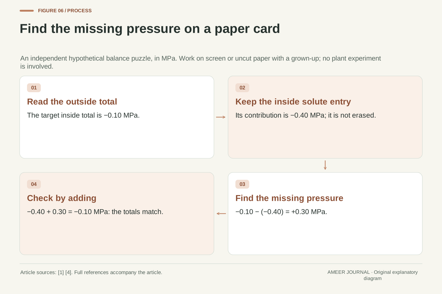
Try one last paper or screen card with your grown-up. The outside total is −0.10 MPa, and the inside dissolved-material entry is −0.40 MPa. Leave the inside pressure entry blank. What number would make the inside total equal the outside? Adding +0.30 MPa works: −0.40 + 0.30 = −0.10. The method is the same two-entry sum, used in reverse. [1][4] The solute entry stayed on the page throughout the calculation; balancing the total did not erase it.
Point to the membrane label, the two inside entries and the outside total as you explain your answer. Then say what the answer leaves unknown: the drawing does not give an actual cell's volume or the time needed for water to move. You may keep the page private and stop after the part that interests you. There is no score or information to submit. A useful explanation is that pressure can balance the solute contribution while dissolved material remains, so zero mean net water gain does not require an empty or motionless cell.
For the final independent card, the two-term balance requires Ψp,in = Ψout − Ψs,in. Substituting −0.10 and −0.40 MPa gives Ψp,in = +0.30 MPa. Check the result by recomputing the sum, rather than by matching a sign alone. [1][4] The exterior value is already a total; it must not be counted again as an extra inside pressure term. This reverse calculation identifies the pressure contribution required for water equilibrium under the stated reduced model.
The card does not adopt the earlier invented wall law, so its solved pressure does not determine x or an absolute volume. Recovering volume would require further constitutive and composition information; recovering a time course would require transport information as well. The optional shared-reading task is an untimed explanation, not a test of a child's ability or an invitation to collect data. The completed argument keeps three ideas together: the membrane defines what can cross, the full relevant potential difference governs passive direction, and equal totals can coexist with unequal component values and retained solutes.
Sources & further reading
Explore the references behind this guide. External pages may change after our review.
- 30.5 Transport of Water and Solutes in Plants - Biology 2e | OpenStaxOpenStax / Rice University · Accessed 7 Nov 2026
- 5.2 Passive Transport - Biology 2e | OpenStaxOpenStax / Rice University · Accessed 7 Nov 2026
- 510 Assignment #4 | Plant Ecophysiology GroupColorado State University · Accessed 7 Nov 2026
Article updated 7 Nov 2026.