What you’ll take away
- Parallel command support does not create independent work that an application has not supplied.
- More outstanding requests can increase aggregate throughput while leaving each request’s latency unchanged or higher.
- Request size and byte units belong beside every IOPS or bandwidth comparison.
- A configured queue limit, observed outstanding count, and lower-level device queue are different quantities.
- Interpret averages and tail latencies with sample counts, workload conditions, and a stated measurement boundary.
A faster total does not necessarily shorten one request
A storage result can show more completed operations per second without showing that each operation finishes sooner. That is not a contradiction. A system can keep several requests in progress and finish more of them overall, while the time each request spends in the system stays the same or increases. SNIA describes this latency-versus-throughput trade-off when discussing queue depth. NVMe is designed to support parallel command submission and completion, but that ability does not tell you how many independent requests your application has available. A large peak result therefore needs its workload conditions before it can explain a shorter wait in your own task. [1][5]
The useful question is what must finish before the application can continue. In an imagined task, each read might reveal where the next read should go. Another task might already know the addresses of many independent reads. Those are different workloads even if they use the same drive. The examples below deliberately separate a request’s completion time, the number of requests in progress, and the total bytes completed per second. They are calculated models, not tests of an SSD. The goal is to identify which measurement explains the work that must finish before the application can continue.
Completion rate and per-operation response time are distinct observables. A workload with more independent operations in flight can achieve greater aggregate throughput without reducing the latency of an individual operation. SNIA’s queue discussion explicitly identifies the environment-dependent trade-off between outstanding work, per-I/O latency, and throughput. NVMe provides parallel submission and completion paths, but protocol capability alone does not establish application concurrency, sustained media performance, or a particular latency distribution. A peak IOPS claim is consequently incomplete for an application-level decision unless the associated workload, concurrency, and measurement boundary are retained. [1][5]
Consider two hypothetical dependency structures. In one, an operation’s result determines the next address, limiting that stream to one outstanding request. In another, many addresses are already known and requests can overlap. Neither structure is a claim about a named application; they isolate why the same hardware may be exercised differently. This article develops closed-loop numerical models in which a completed request is immediately replaced, then distinguishes those assumptions from benchmark configuration and observed behavior. It does not infer controller channel count, endurance, cache durability, or real application speed from the arithmetic. Those would require separate evidence at the appropriate boundary.
Count operations, bytes, time, and outstanding work separately
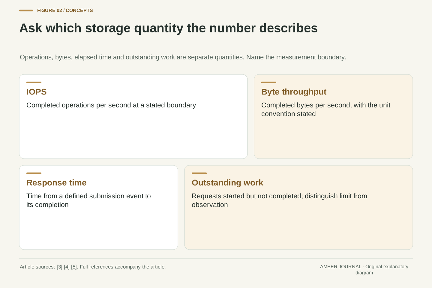
IOPS counts input/output operations completed per second. Byte throughput counts how much data those operations transfer per second. A request’s latency measures time between stated starting and finishing events, while outstanding work counts requests that have started but have not completed at the chosen boundary. Microsoft’s DiskSpd results keep byte totals, bandwidth, operation counts, and latency statistics as separate outputs. That separation matters: one large transfer and one small transfer each count as an operation, but they do not carry the same amount of data. A result stated only in IOPS leaves the request size unanswered. [3][4]
Queue depth needs a similar label. A program can be configured to allow a certain number of outstanding requests, but the configured limit is not automatically a measurement of how many were present throughout the run. The operating system and device also have their own queues. Linux’s block-layer documentation describes software staging and hardware dispatch queues rather than one universal queue shared by every counter. When someone reports a depth of eight, ask where that number came from: a load-generator setting, an observed application count, or a particular lower-level queue. Those descriptions cannot be substituted for each other without checking their scope. [2][3]
IOPS is an operation-completion rate; bandwidth is a byte-completion rate. Latency is elapsed time across a defined operation boundary, while concurrency describes operations outstanding within a defined system boundary. DiskSpd reports per-thread, per-target byte, bandwidth, and IOPS statistics, with latency histograms collected separately when requested. These quantities are related but not interchangeable. If all counted operations transfer the same B bytes, multiplying their completion rate by B gives byte throughput at that same boundary. With mixed sizes, the appropriate total is completed bytes divided by duration, or an operation-weighted size combined with the matching operation rate. [3][4]
A configured outstanding-I/O limit is a control parameter rather than an observed time average. DiskSpd describes issuing operations up to its configured limit and replacing them as completions arrive; scheduling and processing still occur between those events. Linux separately documents software staging and hardware dispatch structures, demonstrating why a queue label must include its layer. The number of allowed commands, submitted commands, waiting requests, and commands currently executing are not automatically identical. Preserve that distinction before using a queue figure in a rate calculation or interpreting it as a direct count of physical flash operations. [2][3]
Build a one-request baseline with explicit assumptions
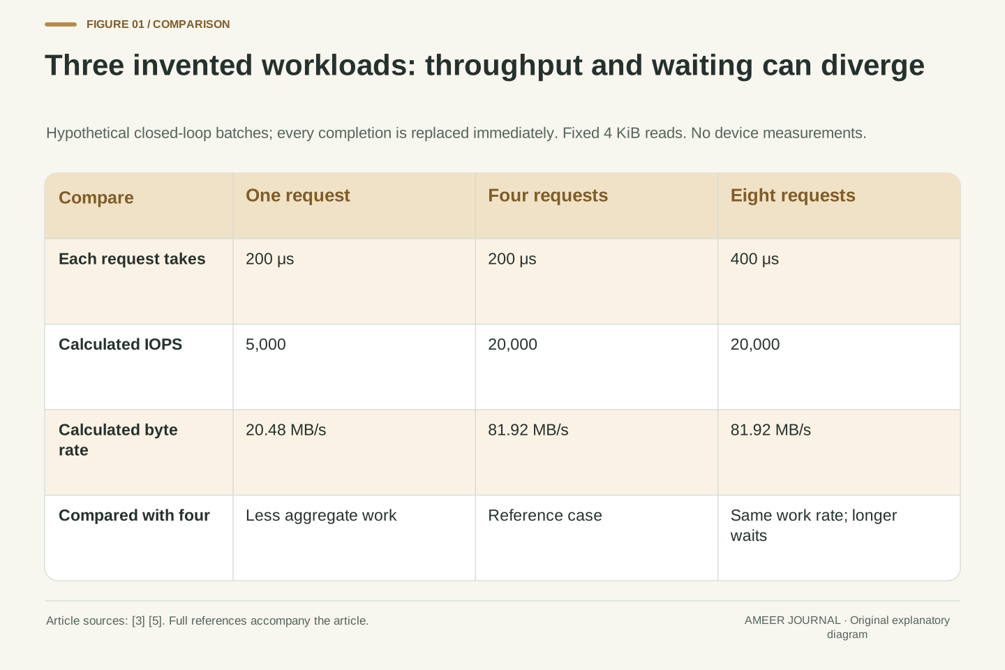
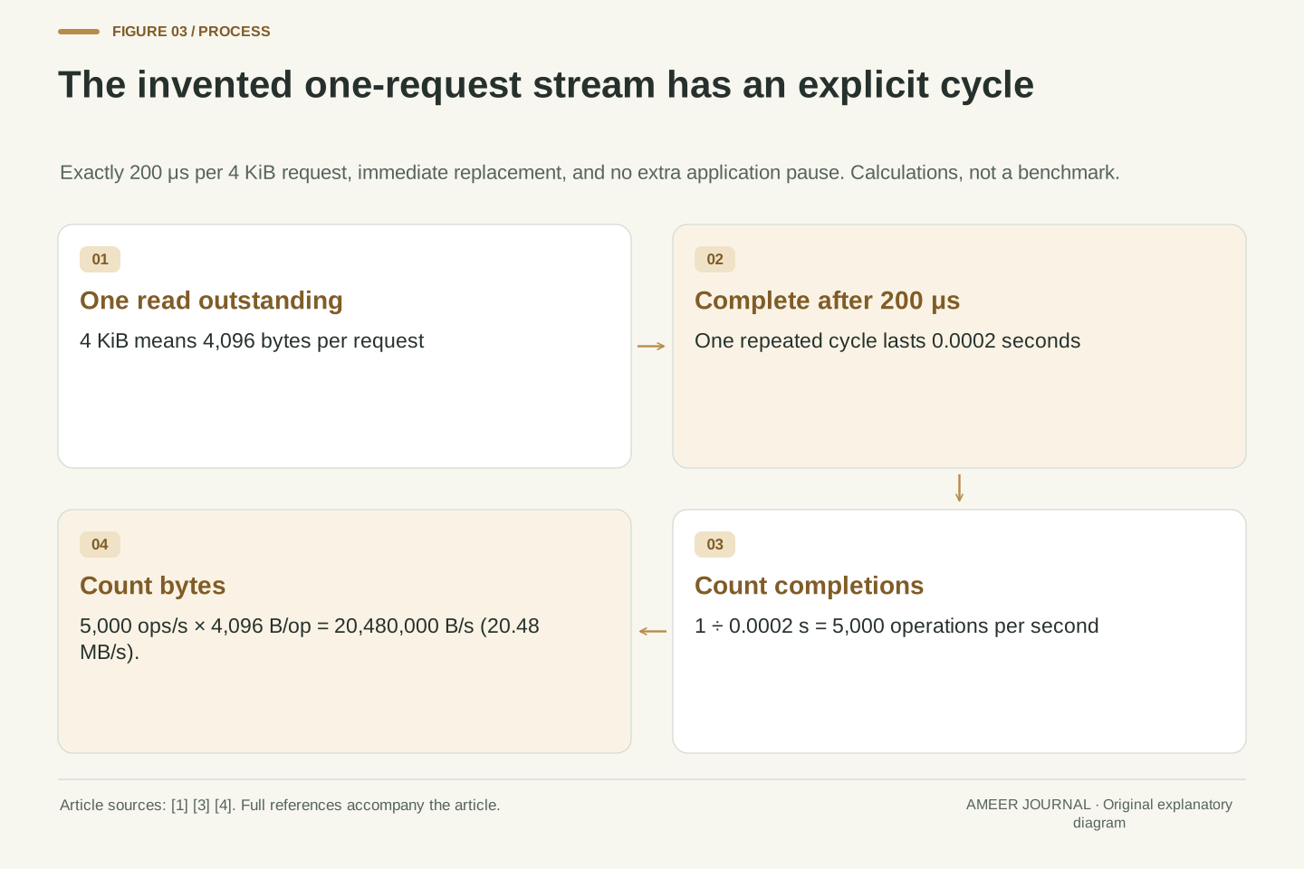
Imagine a workload that keeps exactly one read outstanding. Each read takes exactly 200 microseconds from submission to completion, including everything inside our chosen measurement boundary. The next read is submitted immediately when the previous one finishes, with no extra application pause. Since 200 microseconds equals 0.0002 seconds, this ideal stream completes 1/0.0002 = 5,000 reads per second. If the application then pauses for 50 microseconds before issuing its next read, the complete cycle becomes 250 microseconds. Its rate falls to 4,000 reads per second even though each read still completes in the same 200 microseconds. During the pause there is no request outstanding.
Now give every read a size of 4 KiB, meaning 4,096 bytes. The calculated byte throughput is 5,000 × 4,096 = 20,480,000 bytes per second, or 20.48 MB/s using decimal megabytes. A much larger advertised transfer rate would not change this model unless something about the workload or completion time changed. The example contains only one request to work on at a time. NVMe’s ability to support parallel work cannot manufacture additional independent requests for that stream. Keep this distinction between available concurrency and supported concurrency when comparing an application’s behavior with a high-load benchmark. [1][3]
Define a hypothetical closed-loop stream with one outstanding 4 KiB read, constant submission-to-completion response time W = 200 μs, zero replacement delay, and no other work. Its cycle time is 0.0002 s, so the completion rate is λ = 1/W = 5,000 IOPS. Here W includes the complete declared operation boundary; it is not specifically NAND service time or a controller-only measurement. Startup and shutdown transients are excluded. Adding 50 μs of application think time would make the closed-loop cycle 250 μs and reduce the rate to 4,000 IOPS while leaving the operation’s measured W unchanged. The time-average outstanding population would be 200/250 = 0.8 despite a one-request limit. Response time and complete application cycle time therefore need separate labels.
At B = 4,096 bytes per operation, λB = 20,480,000 B/s = 20.48 decimal MB/s. This figure follows from the invented completion rate and fixed request size; it is not a measured bandwidth ceiling of NVMe or PCIe. A dependent stream that exposes only one request cannot exercise additional command parallelism merely because the interface supports it. SNIA’s NVMe overview establishes that parallel operations are supported, while DiskSpd’s concurrency documentation shows that outstanding-request limits are part of workload construction. Neither source establishes the numerical latency assumed here, which remains an explicit analytical input. [1][3]
Overlap can raise the total without making a request faster
Change the imagined workload so four independent reads start together. Assume the system can complete all four after the same 200 microseconds and immediately start the next four. This grants enough parallel capacity to preserve each request’s completion time, a condition that a queue setting alone cannot establish. Every repeating 0.0002-second cycle now completes four operations, so the rate is 4/0.0002 = 20,000 IOPS. With the same 4 KiB size, the calculated throughput becomes 81.92 MB/s. Each request still waited 200 microseconds. The total increased fourfold, while the individual wait did not decrease.
That is a possible reason for a high-concurrency result to exceed a one-request result, but it is not a promise of fourfold scaling on a real drive. Requests share resources, and the extra load can change their completion times. SNIA explicitly describes that dependence on the storage environment. An application also needs independent work to overlap; changing the benchmark’s request count does not rewrite another application’s dependencies. Read the result as evidence about the tested combination of concurrency and workload. A separate measurement is needed before saying that one interactive operation, file-opening task, or dependent read became quicker. [1][5]
For the second hypothetical system, four independent requests are submitted simultaneously and each completes exactly 200 μs later. All four slots are refilled immediately and the cycle repeats. The completion rate is 4/0.0002 = 20,000 IOPS, with 4,096-byte requests yielding 81,920,000 B/s. The model’s fourfold throughput increase coexists with unchanged per-request response time. This is a constructive example of aggregate progress differing from individual latency. Preserving W requires enough resources under the increased concurrency. If shared resources delay completion instead, the denominator changes and the fourfold rate calculation must be revised.
Increasing a configured depth alone does not establish that invariant response time. SNIA notes that more outstanding operations can increase load on interconnects and storage media and therefore increase per-I/O latency. Application dependencies also bound the concurrency exposed to the stack. Consequently, comparing a low-depth run with a high-depth run answers how that workload behaves under different offered concurrency, not necessarily how quickly a dependent operation finishes. Evidence of improved application responsiveness would require a measurement of the relevant application boundary, with its actual dependency and scheduling behavior retained. Interface support for parallel work is a capability statement, not that measurement. [1][5]
A deeper workload can keep throughput unchanged
For a third invented case, keep eight reads outstanding, but suppose each now takes 400 microseconds. Again, all eight finish together and are replaced immediately. Eight completions every 0.0004 seconds still give 20,000 IOPS and 81.92 MB/s for 4 KiB reads. Compared with the four-request case, twice as many operations are in progress and each waits twice as long, while total throughput is unchanged. The extra occupancy represents more unfinished work inside the measurement boundary, while the rate of finished work stays the same. Looking at both numbers reveals that trade-off immediately.
A comparison that celebrated the bigger queue number would miss the lack of extra completed work. A comparison that looked only at MB/s would miss the longer waits. SNIA’s general guidance describes why lower queue depth can trade some throughput for lower latency, depending on the environment. The sensible question is which result matches the task’s goal: a batch transfer may emphasize total completion, while a dependent request can be held up by its own delay. Even then, evaluate the actual distribution of delays and the full workload, because these deliberately constant-latency examples leave out variation. [5]
Now define a periodic closed-loop batch of eight requests, each with W = 400 μs and immediate replacement at completion. Its λ = 8/0.0004 = 20,000 IOPS matches the four-request, 200 μs case, as does its fixed-size byte throughput. The declared outstanding count doubles and response time doubles, so the quotient is unchanged. The arithmetic checks the relationship among the declared cycle, occupancy and completion rate. To identify whether the longer W came from queue residence, changed service behavior, or another stage, an investigation would need timing at those internal boundaries.
SNIA’s queue discussion supports the qualitative possibility of greater outstanding work increasing latency without a commensurate application benefit. The numerical comparison therefore illustrates why queue depth should be evaluated with both throughput and latency, rather than maximized as a standalone objective. Do not replace the model’s continuously occupied slots with a configured maximum and assume that the same quotient describes a real trace. An observed average, a limit, and a periodically sampled instantaneous count are different quantities. The workload’s dependency structure and latency distribution also determine whether equal aggregate throughput is acceptable for the application. [3][5]
The same byte throughput can require very different IOPS
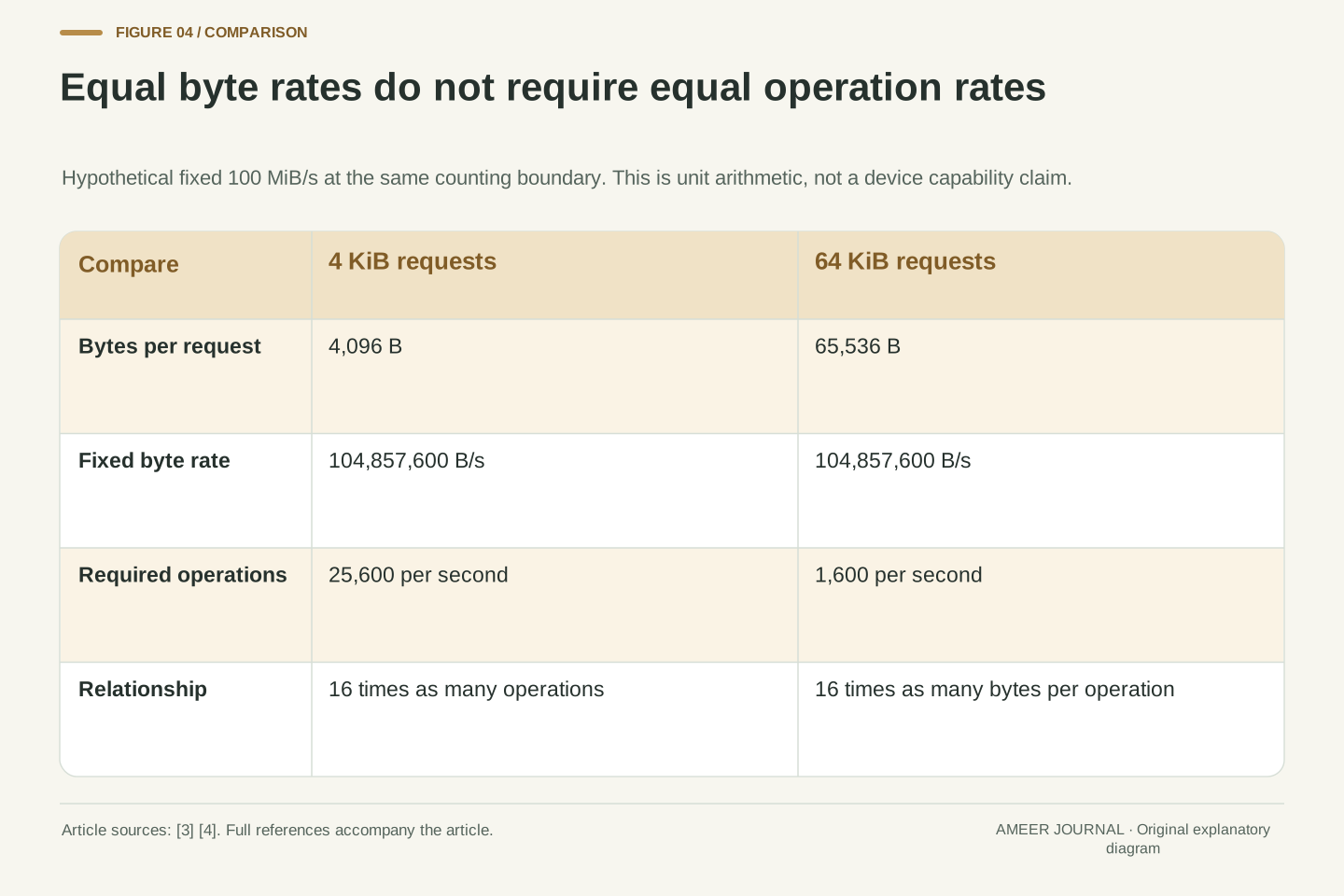
Suppose two hypothetical workloads each transfer exactly 100 MiB every second. A mebibyte, written MiB, contains 1,048,576 bytes, so both transfer 104,857,600 bytes per second. If every operation transfers 4 KiB, divide that total by 4,096 to obtain 25,600 operations per second. If every operation instead transfers 64 KiB, divide by 65,536 to obtain only 1,600 operations per second. The byte throughput is identical, but the operation counts differ by a factor of sixteen. The operation rate changes because each operation carries a different number of bytes.
The reverse comparison also needs care. Keeping IOPS fixed while increasing the bytes per request increases calculated byte throughput only if that operation rate can actually be maintained. Larger requests may change the workload’s timing and resource demands, so a result for small requests cannot simply be multiplied into a promised large-transfer result. DiskSpd’s separate byte and operation statistics help keep the measurements apart. Record the block size and the unit convention beside any reported rate. Decimal MB/s and binary MiB/s describe different numbers for the same byte total; silently switching units can create a difference that is only a conversion. [3][4]
For a fixed-size workload, bandwidth equals completion rate multiplied by bytes per operation at the same boundary. Take an explicitly hypothetical bandwidth of 100 MiB/s = 104,857,600 B/s. At 4 KiB = 4,096 B per request, this requires 25,600 IOPS. At 64 KiB = 65,536 B, it requires 1,600 IOPS. The sixteenfold request-size increase reduces the required operation count by sixteen for this stipulated byte rate. Conversely, the earlier 20,000 IOPS at 4 KiB equals 81.92 decimal MB/s or 78.125 MiB/s; those are equivalent representations of 81,920,000 B/s, not different performance results.
The multiplication is an accounting identity for an observed or stipulated workload, not a device scaling law. Holding λ constant while increasing B requires evidence that the storage path can maintain λ for the changed request size. If it cannot, projecting bandwidth from the old operation rate misstates the new case. DiskSpd’s distinct byte, bandwidth, and IOPS outputs support retaining these dimensions separately. A valid comparison therefore includes request-size distribution, read/write composition, measurement boundary, and unit convention. Mixed-size workloads require total bytes or correctly weighted sizes; an unweighted average of differently scoped metrics does not supply that information. [3][4]
A queue setting may apply to each thread and each target
Microsoft’s DiskSpd documentation gives a specific meaning to its outstanding-request option: the usual -o setting applies per thread and per target. Its -t option sets threads for each target. Imagine a configuration with one target, two threads per target, and eight outstanding requests per thread. Its configured request allowance is 1 × 2 × 8 = 16, not eight. With two targets and the same per-target settings, it becomes 32. These are configured allowances rather than measured queue occupancy. A target can be a file, drive, or partition, so two targets need not mean two physical SSDs. [3]
The documentation also describes fixed-thread and other outstanding-operation controls, so one shortcut does not cover every configuration. Even the number of completions processed together is controlled separately from the number of outstanding requests. This is why a result described only as “queue depth eight” can be ambiguous. Keep the actual tool version and full configuration with the result, including thread and target counts. DiskSpd’s XML output records system and test configuration for this purpose. That record makes it possible to understand what load was offered instead of assuming the label names one universal drive setting. [3][4]
In the documented DiskSpd interface, -o specifies outstanding I/Os per thread per target, while -t specifies per-target threads. A hypothetical one-target configuration with -t2 and -o8 therefore permits 16 outstanding operations across its two threads. Two targets under the same per-target controls permit 32 across four threads. These are configuration-derived counts, not assertions about instantaneous or time-averaged occupancy. Targets can be files, physical drives, or partitions, so target count does not establish physical-device count. The arithmetic applies to the stated option combination and must not be generalized across other ways of constructing threads and outstanding limits. [3]
DiskSpd also documents -F for fixed thread counts, -O for outstanding operations per fixed thread, and -oc for completion dequeue batching independently of the outstanding limit. Those controls demonstrate why an isolated depth number lacks sufficient scope. Preserve the tool version, target mapping, and complete configuration when interpreting an existing result; the option names describe different controls, even when their numerical values happen to match. Microsoft’s results documentation identifies system configuration and full test configuration in XML output. That provenance is necessary to distinguish an interface’s command capacity from the actual workload that generated a reported completion rate. [3][4]
There is more than one place for a request to wait
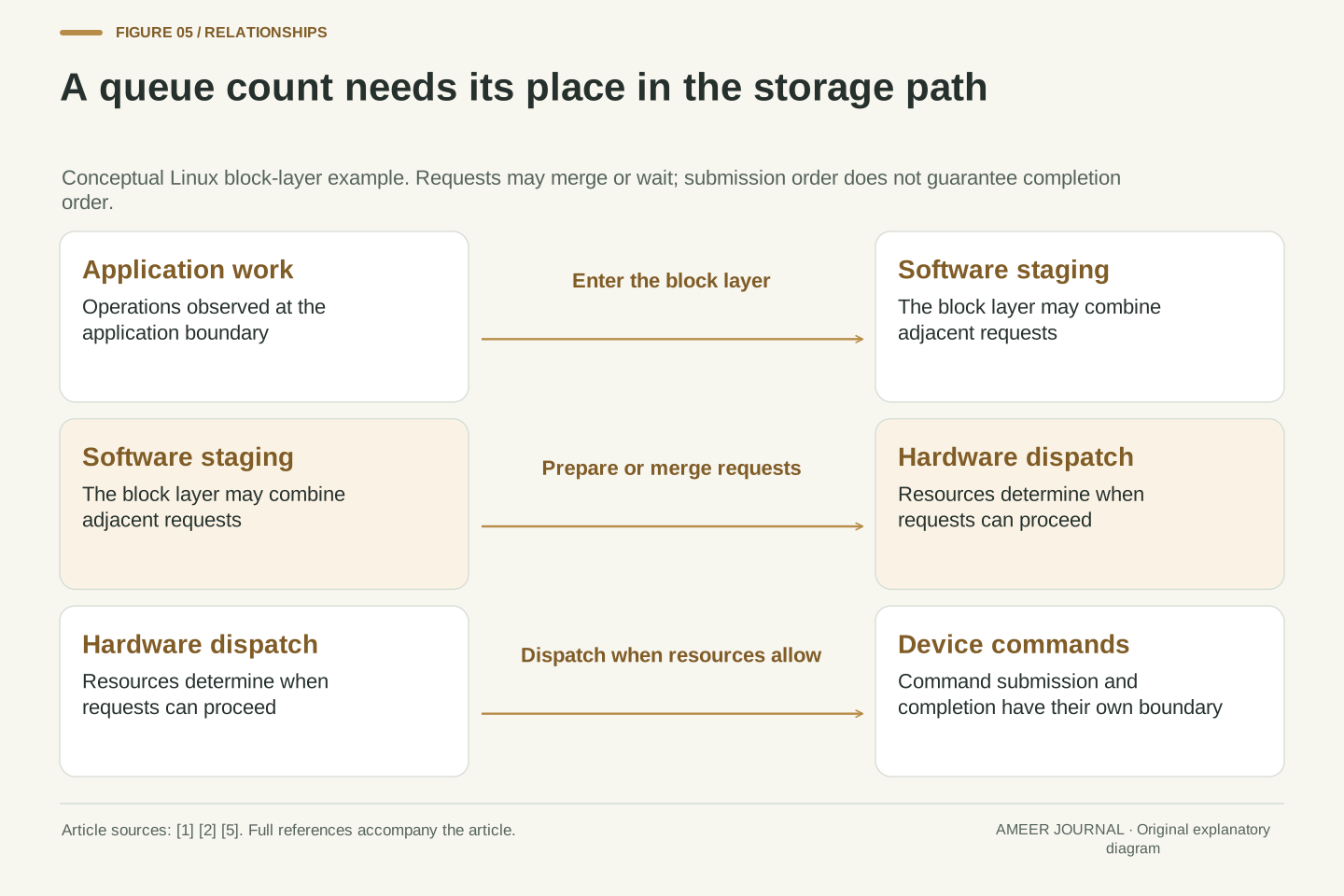
An application’s outstanding work is not necessarily sitting in one device queue. Linux’s multi-queue block layer describes software staging queues, hardware dispatch queues, and requests held until hardware resources become available. It can also combine adjacent requests before dispatch. Those documented mechanisms show why operation counts can depend on where you look. If two higher-level pieces of work are combined lower down, a counter at one boundary need not agree one-for-one with a counter at another. Naming the layer gives that disagreement a concrete explanation to investigate. [2]
Queues and data buffers are different things as well. SNIA distinguishes command/response queues from buffers holding data in flight. A configured count of requests does not by itself tell you the number of bytes in a buffer or the amount of drive cache. Likewise, a queue does not guarantee that completions return in the same order as submissions: Linux explicitly says higher layers must handle completion ordering. For the reader comparing results, the consequence is practical. Preserve whether the reported quantity concerns application requests, block-layer requests, or device commands, rather than treating all three as interchangeable descriptions of a physical line of waiting reads. [2][5]
Linux blk-mq distinguishes software staging structures from hardware dispatch contexts. It can route eligible requests toward hardware, retain requests when resources are unavailable, and merge adjacent work at the staging layer. Its documentation also states that a block request may contain one or more BIOs. These transformations mean that event counts and queue populations must be interpreted at their own boundaries. A userspace operation counter, a block-layer request counter, and a controller-command counter cannot be assumed to describe identical populations. For the documented Linux path, the mapping between those populations is part of the interpretation of each counter. [2]
SNIA separately distinguishes queues containing command/response information from in-flight data buffers. Therefore queue depth is not directly a buffer-byte count or cache-capacity measurement. Linux also warns that completion order is not guaranteed by the block layer or device protocols and must be handled above them. The presence of an ordered submission list should not be interpreted as proof of serial execution or ordered completion. For analysis, retain the event definition, layer, aggregation scope, and time interval alongside each count. Without those details, apparent disagreement between tools may reflect different populations rather than a faulty device or an impossible performance result. [2][5]
An average wait can hide a small group of long waits
Consider two invented sets of 1,000 completed requests. In the first set, every request takes 0.2 milliseconds. In the second, 990 requests take 0.1 milliseconds and ten take 10.1 milliseconds. Both sets have an average of 0.2 milliseconds: the second total is 990 × 0.1 + 10 × 10.1 = 200 milliseconds, divided by 1,000. Yet one percent of the second set waits much longer than any request in the first. These are constructed latency lists, separate from the earlier repeating-workload models. The sum of their response times is not necessarily the elapsed run time because operations can overlap.
Microsoft’s DiskSpd results can report average and percentile latency statistics rather than reducing the run to one mean. Its documentation also warns that high percentiles need enough completed operations to be meaningful: an extreme tail can otherwise depend on only a handful of observations. Keep the sample count, operation type, and duration beside the latency result. A read/write mixture should not be described as though its combined average proved identical behavior for both kinds of request. This does not create a universal acceptable latency target. It gives you enough context to judge whether the measurement answers the application’s actual concern. [4]
Two hypothetical 1,000-operation populations illustrate why the mean is insufficient. Population A has 1,000 latencies of 0.2 ms. Population B has 990 at 0.1 ms and ten at 10.1 ms. Both sum to 200 ms and therefore have a 0.2 ms arithmetic mean, although B contains a one-percent group at 10.1 ms. No percentile interpolation convention is assumed or reported for these lists. Their summed response times are not treated as wall-clock runtime, since concurrent operations can have overlapping durations. The second population concentrates its long waits in ten operations, information that the shared mean removes.
DiskSpd collects latency histograms per thread and target and can report per-operation-type averages and percentile summaries. Microsoft explicitly connects extreme-percentile interpretation to sample size and test duration, noting when there are too few observations to distinguish higher percentiles from the maximum. Consequently, a reported tail statistic should retain operation count, read/write scope, configuration, and duration. A useful comparison also explains its aggregation, rather than assuming that an overall average describes each target or operation class. This evidence can characterize the observed run, but it does not by itself establish a service guarantee or predict all future workload conditions. [4]
Match the result to the task that must finish
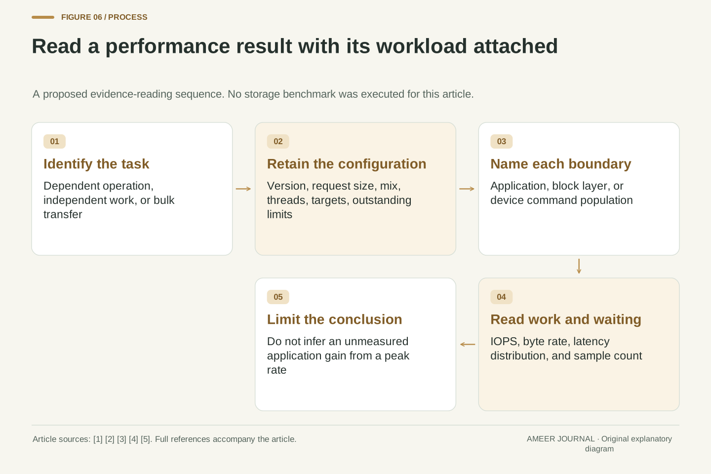
Before using a storage result to explain a real wait, identify the task: one dependent operation, many independent reads, or a large transfer. Then keep the result’s request size, read/write mix, thread and target counts, outstanding-request controls, tool version, and measurement boundary together. Record both the completed work and the delay statistics. Microsoft’s configuration and results documentation shows why these details belong with the numbers. A result with that context can be matched to the task; a headline number with the context removed leaves the relevant comparison unresolved. [3][4]
For the next comparison, ask which assumption changed. Did the system expose more independent requests, shorten their measured completion times, transfer more bytes per operation, or simply use a different unit? If throughput stops improving while waits increase, a larger outstanding count is not automatically progress toward the task’s goal. If a one-request workload remains serial, a result produced with many overlapping requests may answer a different question. NVMe’s parallel design makes concurrency relevant; it does not remove the need to describe it. The useful conclusion is the one supported by the actual workload and its measured completion behavior. [1][3][5]
A defensible interpretation begins with the application’s dependency structure and observable, then preserves workload and configuration provenance. Specify request-size distribution, read/write composition, thread and target mapping, outstanding limits, tool version, and the layer at which counts and response times were observed. Pair throughput with latency distribution and sufficient sample information. Preserving those fields lets a reviewer separate a change in offered workload from a change in the system’s response to that workload. An application completion time, a block I/O response time, and a controller operation rate require separate labels even when they participate in the same storage activity. [2][3][4]
Finally, distinguish what the evidence establishes from what the interface permits. Parallel command support explains why independent requests may overlap, while a higher configured limit establishes only the offered concurrency control. A measured improvement in aggregate work does not establish reduced latency; equal byte throughput does not establish equal operation counts; equal average latency does not establish equal tails. The worked examples isolate each distinction so it can be recognized in a fully documented result. A valid conclusion retains the workload and boundary that produced it, and leaves hardware attribution or application-speed predictions unresolved when the necessary measurements are absent. [1][3][4][5]
Sources & further reading
Explore the references behind this guide. External pages may change after our review.
- What is NVMe? | SNIA | Experts on DataSNIA · Accessed 6 Nov 2026
- Multi-Queue Block IO Queueing Mechanism (blk-mq) — The Linux Kernel documentationThe Linux Kernel · Accessed 6 Nov 2026
- Threading and concurrency · microsoft/diskspd Wiki · GitHubMicrosoft · Accessed 6 Nov 2026
- Analyzing test results · microsoft/diskspd Wiki · GitHubMicrosoft · Accessed 6 Nov 2026
- Buffers, Queues and Caches Explained | SNIA | Experts on DataSNIA · Accessed 6 Nov 2026
Article updated 6 Nov 2026.
Found something we should revisit?
Good explanations get better with thoughtful feedback.