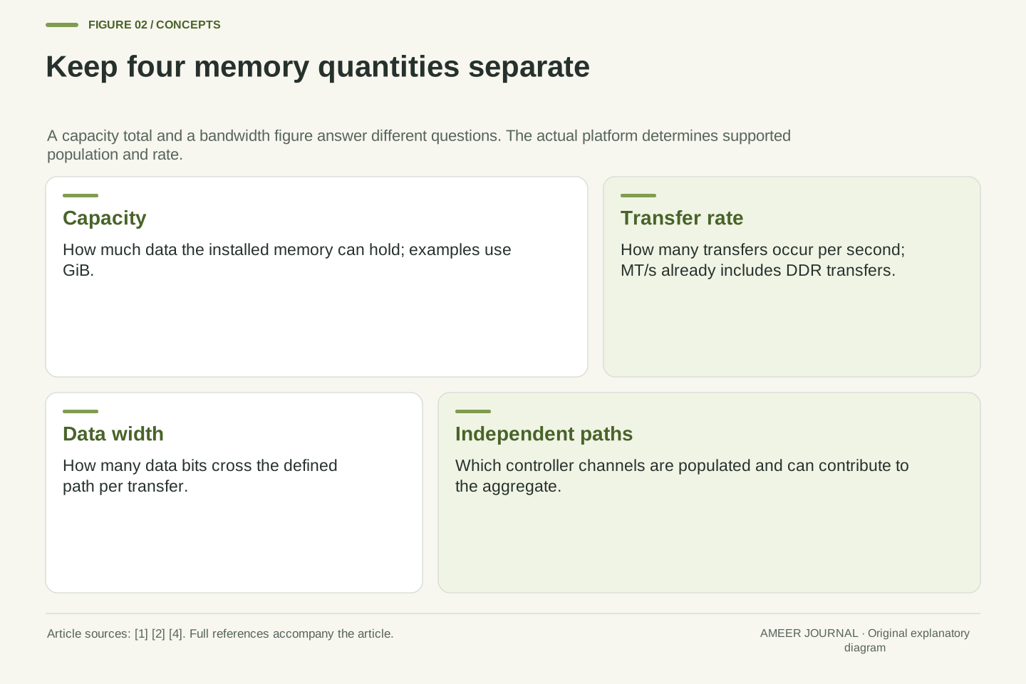
Four memory modules can fill four sockets while still sharing only two memory channels. The modules provide places to store data; the channels provide paths through which the memory controller transfers it. Kingston identifies the belief that four modules automatically produce four-channel performance as a common misunderstanding. On a two-channel platform, adding a second module to each channel increases the installed capacity without creating two additional channels. The supported transfer rate can also change with that arrangement. [4]

This matters when two upgrades look similar on a shopping list. A larger module may give a program more room, while populating another independent channel can increase the theoretical aggregate transfer rate. Filling another socket on an already populated channel does not do the same thing. Start with the processor and motherboard’s channel layout, then ask which channels are populated and at what operating rate. Socket count alone cannot answer those questions. [1][4]

The worked cases below are invented two-channel systems, not installation instructions or measurements of a particular computer. They separate capacity, transfer rate, data width and byte-counting conventions. Actual supported configurations come from the specific platform documentation. Once those quantities are kept distinct, a bandwidth figure becomes a calculation you can inspect rather than a promise that every application will run proportionally faster. [1][4]

Module count and channel count describe different parts of the memory topology. A platform with two channels and two DIMM sockets per channel can contain four DIMMs without exposing four independent controller channels. Kingston’s population guidance explicitly distinguishes one DIMM per channel, or 1 DPC, from 2 DPC and rejects equating four installed modules with quad-channel operation. Population and module organisation can also affect the supported data rate. [4]

The relevant peak-rate model multiplies the effective transfer rate by the data width of each independent path, then aggregates compatible paths. Installed capacity is not another multiplier in that equation. More capacity can change whether a workload fits its available memory, but increasing capacity on an already populated channel does not automatically widen the physical data interface. Conversely, populating an additional independent channel can raise the aggregate theoretical rate even when the total capacity is held fixed. [1][4]

All numerical layouts in this article are original, explicitly assumed examples. They explain arithmetic and measurement boundaries rather than predict a particular motherboard’s configuration or an application speedup. The practical starting point is the actual controller topology, supported population and operating transfer rate. Manufacturer documentation then constrains the example to a real system; a count of visible modules cannot substitute for that information. [1][4]

Memory labels often use MT/s, meaning millions of transfers per second. MHz means millions of clock cycles per second. DDR memory transfers data on both the rising and falling edges of the relevant clock, so the two numbers are not interchangeable. In a simplified interface running at a 1,600 MHz clock, two transfers per cycle give 3,200 MT/s. The transfer-rate figure has already included that doubling. [2]

Suppose a tool reports a 1,600 MHz memory clock while the intended interface rate is 3,200 MT/s. Those values can describe the same operation rather than a memory module running at half its intended rate. The important step is to identify what the tool reports. A clock field, an effective transfer-rate field and a marketing label may use different conventions. Comparing their numbers without the units can produce a false diagnosis. [2]

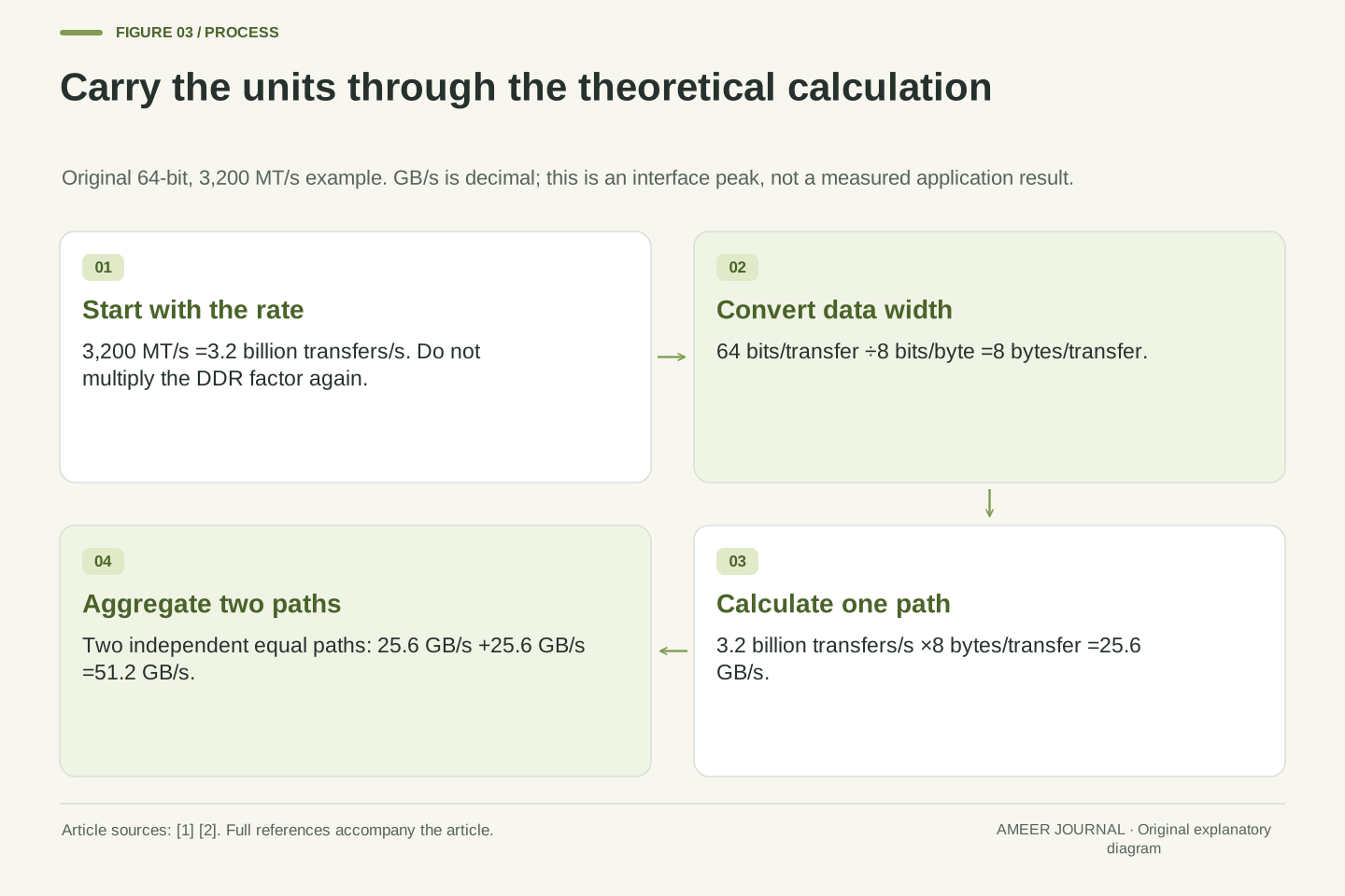
For a bandwidth calculation, start with transfers per second. If the known value is 3,200 MT/s, use 3.2 billion transfers per second directly. Multiplying it by two again would count DDR twice. The width of each transfer still has to be supplied; 3,200 MT/s alone does not state how many bytes travel on the whole interface. That next quantity is what turns an event rate into a data rate. [1][2]

MT/s expresses an effective transfer rate, while MHz expresses a clock frequency. DDR transfers on both clock edges, so an assumed 1,600 MHz interface clock corresponds to 3,200 MT/s. This relationship concerns the relevant external interface clock; it should not be confused with every internal timing domain in a DRAM device. Kingston’s definitions and its clock/transfer-rate examples support the distinction. [2]

If R is already expressed in transfers per second, the DDR factor is already incorporated. A calculation using 3,200×10^6 transfers/s must not introduce a second factor of two merely because the memory is DDR. If starting from the assumed 1,600×10^6 cycles/s instead, multiply by 2 transfers/cycle once. Both routes produce the same R. A diagnostic utility’s field definition determines which route applies; the numeral alone is insufficient. [1][2]

Transfer rate also needs a width boundary. A reported MT/s value does not tell you whether the calculation is for one 32-bit subchannel, a 64-bit aggregate path or several controller channels. Define the data bits carried per transfer before converting to bytes. This avoids two independent errors: counting clock edges twice and counting a width that already aggregates subchannels a second time. [1][2][3]

Assume one channel has a 64-bit data path and operates at 3,200 MT/s. Eight bits make one byte, so 64 bits carry 8 bytes per transfer. Multiplying 3.2 billion transfers per second by 8 bytes per transfer gives 25.6 billion bytes per second. Written with decimal units, that is 25.6 GB/s. Intel’s theoretical-bandwidth explanation uses the same ingredients: rate, width and channel count. [1]

Now assume there are two independent, equally capable channels populated and available to the workload. Their aggregate theoretical rate is 25.6+25.6=51.2 GB/s. That describes the combined data paths. It is not a separate 51.2 GB/s allowance for every core, every application or every module attached to those channels. Sharing the resources does not duplicate the physical interface. [1][4]

Keep the unit convention visible. Here, GB means 1 billion bytes. Expressing the first channel’s 25.6 billion bytes per second in GiB/s, where one GiB is 2^30 bytes, gives about 23.84 GiB/s. Those two figures can represent the same rate. A smaller number on a display is not necessarily a slower system if the display uses a different unit. First match the bytes being counted and their units, then compare the result.

For an assumed data width W=64 bits/transfer and effective rate R=3.2×10^9 transfers/s, the theoretical data rate is B=R×W÷8 bits/byte. Substitution gives 3.2×10^9×64÷8=25.6×10^9 bytes/s, or 25.6 GB/s in decimal units. The transfer and bit units cancel explicitly. Intel’s Core X-Series support note illustrates this rate-width-channel method, although its particular processor example is not the hypothetical platform used here. [1]

Two independent paths with that same width and rate yield Btotal=ΣBi=51.2 GB/s. Aggregation assumes the defined channels can contribute; it does not assign the aggregate peak to each thread or DIMM. Nor should separate read and write labels be casually treated as proof of two independent buses with twice this aggregate. Define the interface and traffic accounting before making such a claim. The calculation is a physical data-path ceiling, not an application-throughput observation. [1][4][5]

Decimal and binary scaling are another independent boundary. 25.6×10^9 bytes/s divided by 2^30 bytes/GiB is approximately 23.8419 GiB/s. A result expressed as 25.6 GB/s and one expressed as 23.84 GiB/s need not disagree. Capacity examples below use GiB deliberately, while transfer rates use decimal GB/s. Retaining those units also prevents a capacity label from being mistaken for an extra bandwidth factor.

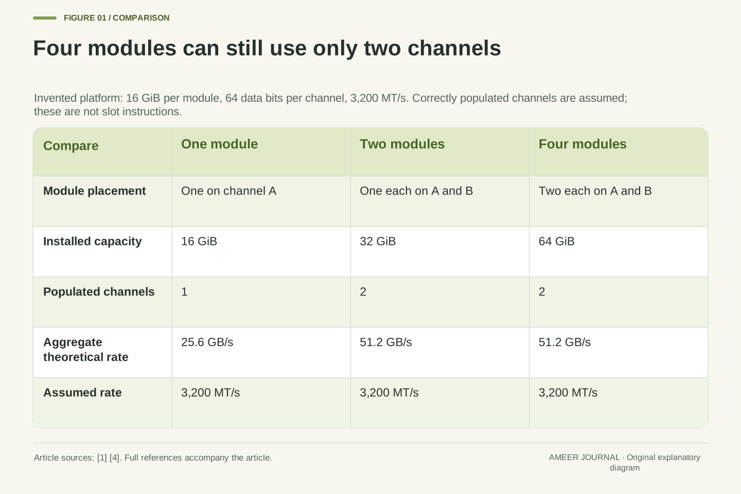
Imagine two channels, A and B, each with two sockets. Every module in the example holds 16 GiB. One module on channel A provides 16 GiB of capacity and one populated data path. At the assumed 3,200 MT/s rate and 64-bit width, its theoretical rate is 25.6 GB/s. This is a drawn example, so the socket labels do not prescribe which physical slot to use on a real motherboard. [1][4]

Put a second 16 GiB module on that same channel A. Capacity becomes 32 GiB, but the example still has one populated channel and the same 25.6 GB/s peak at the unchanged rate. Instead, put one 16 GiB module on A and one on B: capacity is also 32 GiB, while the two populated paths can provide 51.2 GB/s in aggregate. Equal installed capacity can therefore coexist with different channel utilisation. [1][4]

Finally, populate all four sockets with 16 GiB modules. Capacity reaches 64 GiB, but the controller still has two channels. If both keep the assumed 3,200 MT/s rate, the same aggregate 51.2 GB/s ceiling applies. The extra modules may affect other aspects of operation, but four modules do not become four independent channels through arithmetic. For actual placement and support, use the motherboard’s population instructions rather than the drawing. [4]

Define an invented topology with channels A and B, two sockets on each channel, a 64-bit aggregate data width per channel, and 16 GiB per DIMM. Hold the operating rate at 3,200 MT/s for this comparison. A single populated A socket gives 16 GiB and 25.6 GB/s theoretical bandwidth. This explicitly separates the count of addressable bytes from the count of populated independent data paths. [1][4]

A second DIMM on A doubles the assumed capacity to 32 GiB without changing the one-channel peak. Moving that second module to B leaves capacity at 32 GiB but populates a second path, so the aggregate rises to 51.2 GB/s. This is a topology comparison at equal capacity and rate, not an assertion that every actual controller supports an arbitrary unbalanced layout or that it maps every workload across channels in the same way. [1][4]

Populating both sockets on both channels produces 64 GiB at 2 DPC. The number of channels remains two, and at the held rate the aggregate stays 51.2 GB/s. Kingston’s guidance describes the same 1 DPC-versus 2 DPC distinction and warns that extra population can reduce the supported operating rate. The fixed-rate example isolates topology first; the next example removes that assumption. Neither a module count nor a capacity total identifies the complete configuration. [4]

The label on a memory module is not the whole system’s operating contract. The processor, motherboard, module organisation and population can restrict the supported transfer rate. Kingston’s tables are organised around those variables and direct readers to the specific motherboard documentation and supported configurations. Adding modules can therefore change more than capacity. Check the rate the resulting system actually supports and uses. [4]

Take the two-channel example with 32 GiB and a 51.2 GB/s peak at 3,200 MT/s. Now imagine adding two modules gives 64 GiB, but this fictional platform then operates at 2,400 MT/s. Each channel’s peak becomes 2.4 billion transfers/s×8 bytes/transfer=19.2 GB/s, so the total is 38.4 GB/s. Capacity doubled while theoretical bandwidth fell by 25 percent. Those are separate changes, and neither can be inferred from the other.

This does not tell you which configuration is better for an actual task. A workload that needs the additional capacity asks a different question from one that already fits and spends its time moving data. The example also does not predict that a real machine will choose 2,400 MT/s. Its purpose is to show why a calculation must be repeated after a change in operating rate, instead of carrying the old bandwidth figure into a new configuration. [1][4]

Supported rate is a property of the assembled platform and configuration. Kingston’s population guidance includes processor and chipset constraints, module rank organisation, and 1 DPC or 2 DPC layouts; it directs the reader to motherboard documentation and qualified configurations. A module capability or profile is therefore not sufficient evidence that the memory controller will operate the populated system at that same rate. [4]

In the original downclock scenario, two 64-bit channels at 3,200 MT/s have a 51.2 GB/s peak. After increasing capacity from 32 GiB to 64 GiB, assume the permitted operating rate becomes 2,400 MT/s. Recompute B=2×2.4×10^9×8=38.4×10^9 bytes/s. The ratio 38.4/51.2=0.75 gives a 25 percent reduction in peak rate while installed capacity increases 100 percent. The 2,400 MT/s value is a constructed condition, not a processor support table.

Capacity sufficiency and bandwidth demand must consequently be evaluated separately. The phase model later in this article considers rate-sensitive work, but it cannot answer what happens when the smaller configuration cannot hold a workload’s required data. For a real comparison, retain the actual operating rate and population alongside capacity, then investigate the workload. This avoids treating a bigger capacity label as evidence of either a faster or a slower complete application. [1][4][6]

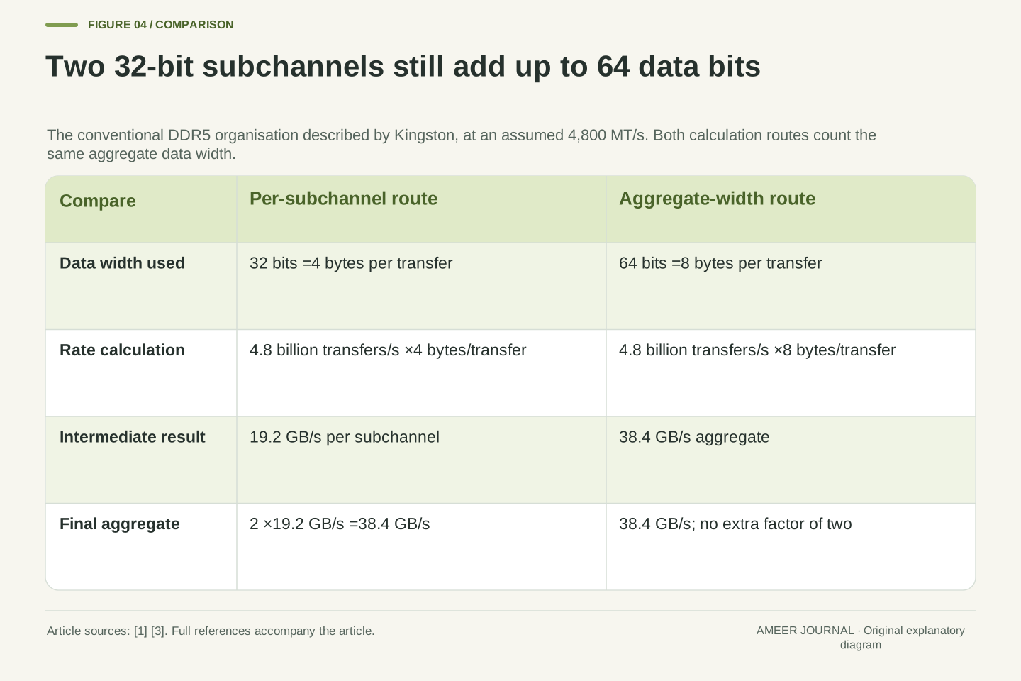
DDR5 introduces another naming trap. Kingston describes a conventional DDR5 module with two independently addressable 32-bit subchannels while the aggregate data width remains 64 bits. Splitting the path changes how the controller can organise accesses; it does not turn 64 data bits into 128. Count either two 32-bit paths or one 64-bit aggregate for that module boundary, then use that choice consistently. [3]

At an assumed 4,800 MT/s, each 32-bit subchannel carries 4 bytes per transfer and has a 19.2 GB/s theoretical rate. Two such subchannels total 38.4 GB/s. Calculating 4.8 billion transfers/s×8 bytes/transfer gives the same 38.4 GB/s directly. Multiplying that result by two again just because the module has two subchannels would double-count the width already included in 8 bytes. The labels differ; the arithmetic must preserve the same physical data path. [1][3]

This example concerns the 64-bit module organisation described in the source, not every possible DDR5 product or memory system. Kingston also describes additional bits used for ECC on server modules. Those check bits should not be counted as extra application-data bytes in this particular data-bandwidth calculation. When specifications use “channel” at different levels, write down the width and boundary first. That is safer than assuming every occurrence of the word identifies another complete 64-bit path. [3]

Kingston’s DDR5 overview describes two independent 32-bit addressable subchannels within an aggregate 64-bit data organisation. The calculation can be expressed per subchannel or at the aggregate boundary. These are two descriptions of the same width, not independent multiplicative benefits. Subchannel scheduling can affect efficiency without changing 64 data bits into 128 data bits. Restrict that explanation to the documented module organisation rather than universalising it to every form factor. [3]

At R=4.8×10^9 transfers/s, Bsub=R×32/8=19.2×10^9 bytes/s. Summing two subchannels gives 38.4 GB/s. Equivalently, Baggregate=R×64/8=38.4 GB/s. Applying another factor of two to the 64-bit aggregate would count the same subchannels twice. If a system genuinely supplies another independent 64-bit aggregate path at the same rate, that additional path can contribute separately, giving 76.8 GB/s across the two defined aggregates. [1][3][4]

The source’s server-module discussion includes extra ECC bits on each subchannel. Those physical check bits are not additional user-data payload in the 64-bit data-width model used here. Likewise, labels referring to module organisation should not be turned into extra simultaneously independent data paths without establishing the controller boundary. Record data width, subchannel count and aggregation convention explicitly; this makes a comparison interpretable even when different specification tables use channel terminology differently. [3]

A theoretical rate assumes the data paths can keep transferring at the stated rate. A program also has to request useful data in a way the system can supply. Intel’s bandwidth note lists workload and system-state factors that can lower observed bandwidth. Its separate optimisation example shows why the order of memory accesses and the way data fits in cache matter. A large peak figure alone does not describe that access pattern. [1][6]

Cache adds another boundary. Data used repeatedly may be supplied from a cache rather than fetched again from main memory. Intel’s worked optimisation recipe explicitly examines traffic at different levels and describes reducing DRAM traffic by doing more work with cached data. That can improve the application while lowering the amount of data crossing the DRAM interface. A smaller DRAM-traffic number is therefore not automatically evidence that the program has become slower. [6]

Ask what the measurement represents: a physical interface peak, sustained traffic through main memory, traffic served by cache, or completed application work. These quantities can move differently after an optimisation. STREAM was designed to measure sustained bandwidth using simple vector workloads and data sets that exceed cache capacity. Its result answers a defined workload question; it does not replace every application’s own performance measurement. [5]

The rate-width calculation describes an interface ceiling; sustained performance also depends on whether requests exercise that interface effectively. Intel’s theoretical-bandwidth note identifies workload and power-state variability. Its 2023 Advisor recipe examines access patterns, locality and cache blocking in a specific matrix computation. The mechanism is relevant here, while that recipe’s timing improvements are not transferred to an unrelated machine or program. [1][6]

Memory hierarchy boundaries matter because requested application bytes need not all traverse DRAM. Reuse in cache can reduce external memory traffic. Intel’s recipe explicitly describes a later state with less DRAM traffic and more cache-level traffic as the intended optimisation. Consequently, observing a lower DRAM byte rate does not by itself determine whether useful computation decreased. Establish the numerator and the measurement level before interpreting bandwidth as a success metric. [6]

STREAM’s reference describes sustainable bandwidth for simple vector kernels and distinguishes main-memory measurement from cache-bandwidth measurement. Its data-size requirements are designed to avoid representing a cache-resident test as main-memory bandwidth. The general principle is to match the tested working set and access pattern to the claim. A benchmark can characterise a particular sustained workload without establishing latency for every access pattern or throughput for every application. [5]

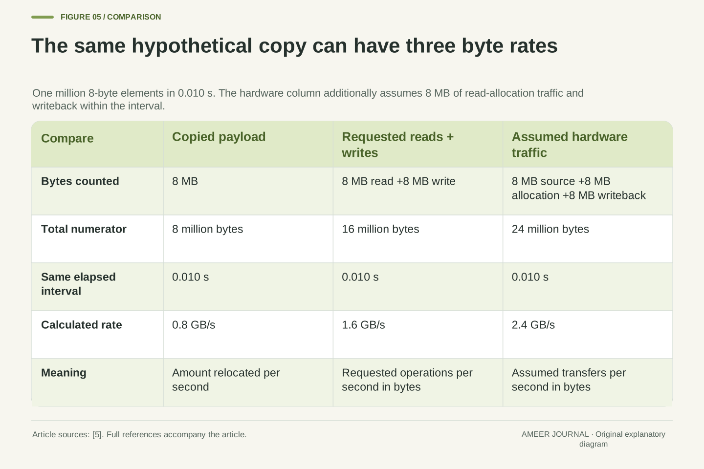
Imagine a hypothetical copy that moves 1 million elements, each 8 bytes, in 0.010 seconds. The copied payload is 8 million bytes. Dividing that payload by the elapsed time gives 800 million bytes per second, or 0.8 GB/s. But a convention that counts both the requested read and the requested write counts 16 million bytes and reports 1.6 GB/s for the very same copy. Nothing became faster between those two calculations; the numerator changed. [5]

STREAM’s reference explains this distinction and also separates requested bytes from hardware traffic. For one further invented case, assume the hardware reads 8 MB of source data, reads 8 MB of destination data into cache before overwriting it, and writes 8 MB back within that same interval. That assumed 24 MB of traffic gives 2.4 GB/s. Real traffic depends on the cache state and store method, so this third number is a stated example rather than a rule for every copy. [5]

All three values can therefore be mathematically consistent: 0.8 GB/s of copied payload, 1.6 GB/s of requested reads plus writes, and 2.4 GB/s of the assumed hardware traffic. A comparison becomes misleading if their labels disappear. Before declaring that one memory system is twice as fast, check whether both reports counted the same work, across the same boundary, over the same interval and with the same unit convention. [5]

For an original copy example, let N=1,000,000 elements, element size 8 bytes, and elapsed time t=0.010 s. A payload convention counts 8,000,000 bytes and yields 0.8 GB/s. A requested-read-plus-write convention counts 16,000,000 bytes and yields 1.6 GB/s. STREAM’s reference distinguishes these conventions: its Copy accounting includes both requested loads and stores, whereas its described bcopy convention counts the amount relocated once. [5]

A third, explicitly assumed hardware case includes an 8 MB source read, an 8 MB destination read-for-allocation, and an 8 MB destination writeback, all occurring within t. Then 24,000,000/0.010=2.4×10^9 bytes/s. The write-allocation mechanism is described in the reference, but this complete traffic schedule is hypothetical. Existing cache contents, store policy and when writeback occurs can change physical traffic within a measured interval. No universal 24-byte-per-element claim follows. [5]

The three rates differ by accounting boundary, not by elapsed execution time. For comparison, retain whether the numerator represents copied payload, requested operations, or observed hardware transfers. Also retain units and interval boundaries. A counter-based DRAM measurement and an algorithm-level byte count are not automatically interchangeable, even when both tools print GB/s. Agreement or disagreement becomes meaningful only after the counted events are defined. [5][6]

Suppose a fictional task takes 1.0 second. In our deliberately simple model, 0.4 seconds is work that will not change, and 0.6 seconds is a separate phase whose time is limited entirely by memory bandwidth. Assume the phases do not overlap. If usable bandwidth for that second phase doubles, its time falls to 0.3 seconds. The whole task then takes 0.4+0.3=0.7 seconds, not 0.5 seconds.

That is a 30 percent reduction in elapsed time. For repeated identical tasks, the corresponding throughput factor is 1/0.7, about 1.43 times, or 42.9 percent more tasks per second. Those percentages describe different quantities. The model is generous to the bandwidth improvement because it assumes the entire 0.6 second phase scales perfectly. A change in the theoretical interface peak alone does not establish that the usable rate for that phase doubled. [1][6]

The calculation gives you a question to investigate: how much of this task can actually benefit from the change? If the program mostly reuses cached data or waits on something else, the answer can differ from a streaming copy. If extra capacity changes the workload’s behaviour, that is another mechanism again. Compare the complete task you care about while preserving its inputs and conditions, then use the memory figures to explain the result. [5][6]

Use an idealised sequential-phase model with Tfixed=0.4 s and Tbandwidth=0.6 s, giving Tinitial=1.0 s. Assume fixed work, no phase overlap, no other behavioural change, and an actual doubling of usable bandwidth for the bandwidth-limited phase. Then Tnew=Tfixed+Tbandwidth/2=0.7 s. This arithmetic isolates the fraction of runtime that can scale; it is not a benchmark or a prediction from channel count alone.

The elapsed-time reduction is (1.0−0.7)/1.0=30 percent. For repeated identical tasks under the same model, the throughput ratio is 1.0/0.7≈1.4286, corresponding to 42.86 percent higher throughput. Distinguish these quantities rather than reporting a vague 43 percent faster result. Most importantly, a doubled theoretical peak is not the same premise as doubled usable bandwidth for the relevant phase. Workload and access-pattern evidence is required to connect those claims. [1][6]

The model also holds the working set and capacity sufficiency fixed. It does not describe a capacity upgrade that changes whether the task can operate as before. Cache reuse, traffic reduction and non-memory work require their own analysis. Use the measured complete-task outcome as the result, then investigate which mechanism changed. That order prevents a specification-sheet improvement from being promoted directly into an application-performance claim. [4][5][6]

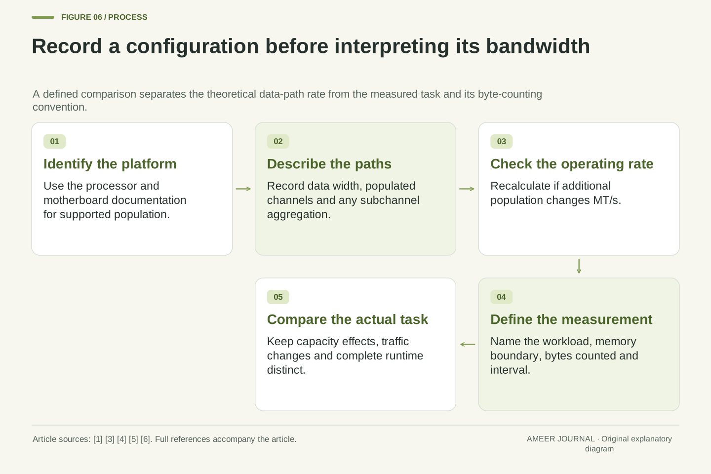
A useful memory-bandwidth record begins with the processor and motherboard, the supported configuration, the installed module capacity and the sockets used. Add the operating transfer rate, the data width convention and the number of populated independent channels. Those details let someone reconstruct the theoretical calculation and see whether two systems really use the same boundary. The platform manual matters more than an assumption based on the number of modules visible through a case window. [1][3][4]

For a measured result, also record the task, data-set size, byte-counting convention and elapsed interval. State whether the claim concerns main memory, cache or total application time. A STREAM-style result should identify the actual benchmark and its relevant run conditions; an invented calculation should remain labelled as one. This separates an interface specification from a result that someone could reproduce. [5][6]

Return to the original four-module question. More modules may supply more capacity, populate additional channels, share existing channels, or change the supported operating rate. Determine which of those happened before predicting the effect. Then compare the workload using consistent measures. The most useful bandwidth number is the one whose paths, units, configuration and counted work are all clear enough to check. [1][4][5]

Retain a topology-and-rate record: platform identity, supported population, module organisation and capacity, populated channels, data width boundary and actual operating rate. Compute each independent path and aggregate only the intended paths. For DDR5, specify whether a figure is per 32-bit subchannel or per 64-bit aggregate. For ECC-capable organisations, keep check-bit width distinct from the user-data-width calculation. [1][3][4]

Retain a separate measurement record: workload and implementation, data-set size relative to the relevant cache, counting convention, interval, units and system state. STREAM’s reference distinguishes standard and modified results and explains why its reported bytes need not equal hardware traffic. A result with those details can support a defined comparison; a bare GB/s label cannot establish that two runs measured the same thing. [5][6]

The interpretation then becomes concrete. Capacity is the amount stored; effective transfer rate and width determine a theoretical path rate; populated independent paths determine the aggregate; the workload and measurement boundary determine what was observed. Four DIMMs on two channels remain a two-channel population. Whether that arrangement is useful depends on its supported rate, required capacity and actual task, rather than a universal rule that each extra module multiplies bandwidth. [1][4][5][6]