Your computer shows a gigabit Ethernet connection, yet a file-copy window displays a much smaller number. Both can be correct. One describes a link; the other may describe useful file bytes arriving during a timed operation. Before looking for a fault, identify what each number counts, which direction it covers and whether the units are bits or bytes. Comparing the labels is the first part of comparing the speeds.

The distinction exists in technical reporting too. Microsoft’s interface structure has separate transmit-link and receive-link speeds, measured in bits per second, alongside counters for data that actually passed through the interface. The Ethernet reporting model in RFC 3635 also distinguishes operational speed from duplex mode. A reported capability while a link is not yet operational needs different interpretation from an established connection’s speed. [1][2]

We will use one established Ethernet link rated at 1,000,000,000 bits per second, without combining links. The packet sizes, busy-path example and transfer result are constructed cases. They show which information connects a local capability to an application result; they are not measurements of a particular network.

A link-rate report and an application-throughput report can describe different populations of bits over different boundaries. The former describes an interface’s operating rate; the latter may count unique file bytes delivered over an interval. RFC 5136 makes protocol layer and measurement interval central to capacity definitions. Without those labels, a numerical comparison can combine physical, link, network and application quantities as though they were interchangeable. [3]

Microsoft’s MIB_IF_ROW2 separates TransmitLinkSpeed and ReceiveLinkSpeed, in bits per second, from received and transmitted octet counters. RFC 3635’s Ethernet interface model likewise distinguishes speed and duplex; its pre-negotiation reporting rule can expose a supported maximum before an operational speed exists. [1][2] These are documented reporting examples, not an assertion that every operating-system screen reads the same field or uses identical display conventions.

The analytical cases below assume one established, unaggregated 1 Gb/s Ethernet link, with decimal units throughout. Packetization, loads and timings are stipulated rather than measured. The path and TCP examples identify their own layer boundaries. This lets us examine three separate questions: what the local interface can carry, what remains available across the path, and what the chosen application actually delivers during its timed work.

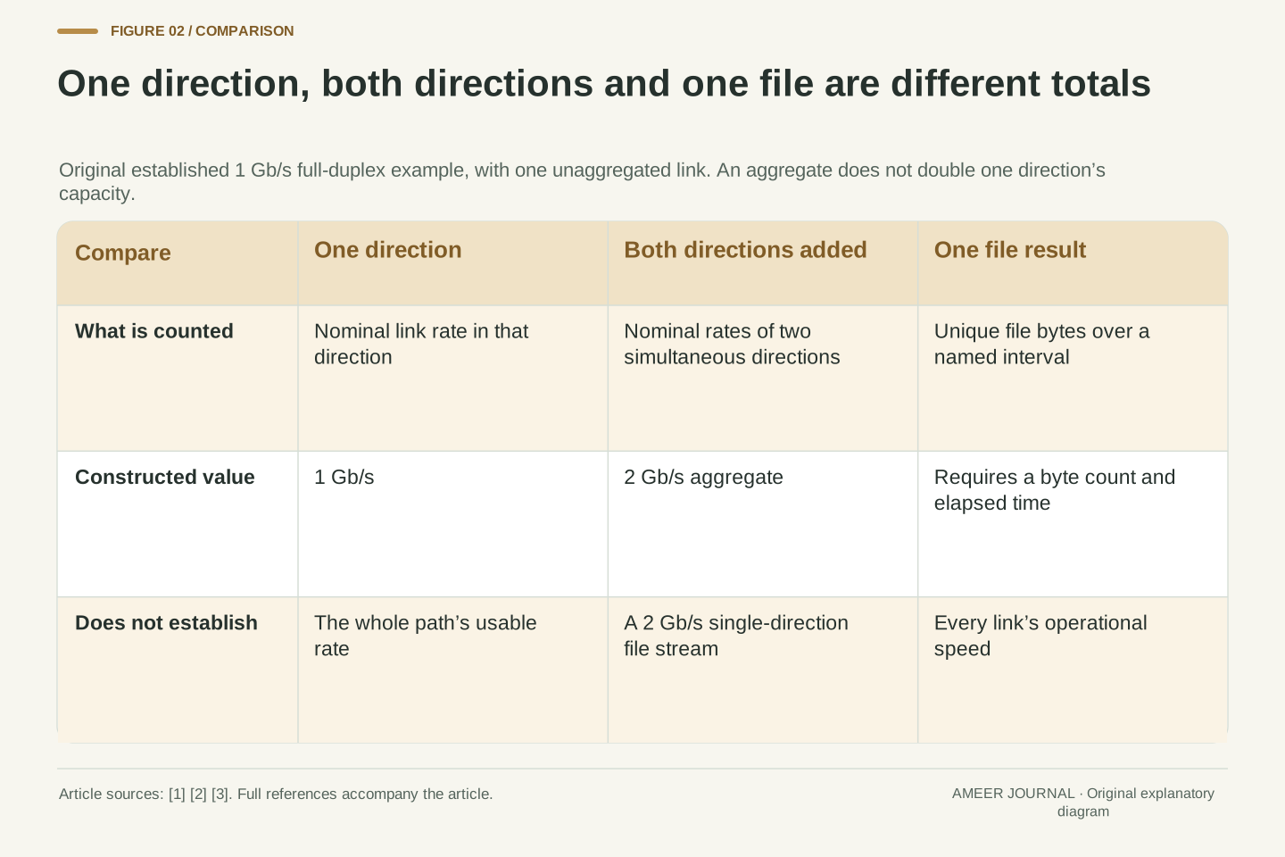
Full-duplex communication allows the two ends to send and receive at the same time. For the gigabit link in our example, there is a nominal gigabit-per-second direction from the computer and another toward it. Adding them describes two directions working together. It does not turn a single download into a two-gigabit stream. RFC 3635 explicitly says its Ethernet speed objects must not double the line-speed value merely because the interface is full duplex. [1]

This also helps you read a switch specification that describes an aggregate rather than one transfer. First ask which ports and directions are being added. A total can be meaningful without being the capacity available to one file going from one sender to one receiver. Microsoft’s separate transmit and receive speed fields are another reminder to keep the direction attached to the number. [2]

TCP adds a related distinction: a receiver sends acknowledgments about data it has received. Those return messages belong to the opposite direction on this simple full-duplex link. Their existence does not mean every acknowledgment must consume the forward direction’s transmission time. But the return path and acknowledgment timing can still affect the TCP conversation, as the later window example explains. Separate physical directions do not make the two ends of a reliable transfer independent. [4][5]

Full duplex supports simultaneous transmission and reception. In the stipulated symmetric 1 Gb/s link, the directional nominal rates are each 1 Gb/s; summing them gives a 2 Gb/s bidirectional aggregate, not a 2 Gb/s forward channel. RFC 3635 explicitly prohibits doubling ifSpeed or ifHighSpeed because of duplex mode. [1] The example assumes one link, so link aggregation and multiple network paths are outside this arithmetic.

A switch-wide aggregate must similarly retain the set of ports and directions being counted. It is not automatically a per-flow capacity. The Microsoft interface structure’s separate transmit and receive rate members provide a concrete reporting example. [2] A useful comparison identifies whether a figure describes one egress direction, both directions of one port, or a larger sum before comparing it with a single application’s byte rate.

TCP acknowledgments travel in the reverse direction of the acknowledged data. On the assumed full-duplex link, reverse traffic does not directly occupy the forward serialization budget. That does not remove transport coupling: acknowledgment timing and the permitted outstanding data affect forward progress. [4][5] The payload calculations later assume the acknowledgment path is adequate. They do not silently charge reverse acknowledgment bytes to the forward channel or claim the return path can never become a constraint.

A local Ethernet connection is one part of a route between applications. A transfer to a nearby storage computer may stay within the local network; a download from a remote server crosses a different path. The access connection alone cannot establish the performance of all the intervening links and endpoints. RFC 6349 makes that limitation explicit in its framework for measuring complete TCP paths. [4]

Consider an invented route with three successive links rated at 1 Gb/s, 100 Mb/s and 1 Gb/s. Even if the first and last links have plenty of room, every byte of this transfer must cross the 100 Mb/s link. Changing only the first connection to a faster one does not remove that limit. This example assumes no other restriction; useful payload will still need its own overhead calculation.

The general rule needs consistent definitions. RFC 5136 defines path capacity at the IP layer using the smallest corresponding link capacity along that path. [3] You cannot take a physical-link label from one device, a useful-file rate from another and treat their minimum as an exact result. For an everyday comparison, begin by identifying the actual sender, receiver and route. A good local result and a slower internet download may be testing substantially different work.

End-to-end capacity concerns the complete path, not only the interface nearest the observer. RFC 6349’s managed-network framework explicitly warns that provisioning an access segment does not establish guaranteed end-to-end performance. [4] A local storage transfer and a remote-server download can differ in route, endpoints and transport conditions even when the observing computer uses the same Ethernet interface for both.

For a constructed serial path with nominal link rates of 1 Gb/s, 100 Mb/s and 1 Gb/s, the 100 Mb/s segment bounds the forward link-rate budget. Under the later full-size, untagged IPv4/TCP model, its corresponding ideal TCP-payload ceiling is about 94.93 Mb/s. That conversion uses the stated framing assumptions; it is not a measured rate or a claim that every 100 Mb/s path delivers that payload throughput.

RFC 5136 formalizes path capacity as the minimum link capacity at the same IP-layer definition and interval. [3] Mixing nominal Ethernet rates with IP capacity or unique application goodput breaks that comparison. The practical record should therefore distinguish the physical route from the accounting layer. Faster hardware on a non-limiting segment may change one local capability while leaving the relevant path constraint intact.

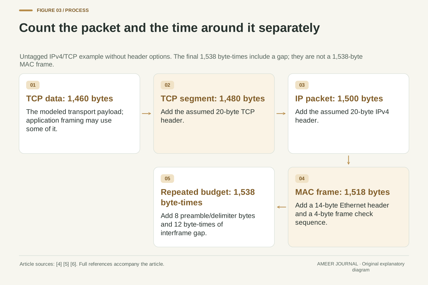
Use a deliberately simple packet: untagged Ethernet carrying IPv4 and TCP, with a 1,500-byte IP packet, a 20-byte IPv4 header and a 20-byte TCP header. There are no header options or extra encapsulations. That leaves 1,460 bytes of TCP data. RFC 6349 uses this restricted model; the IPv4 and TCP specifications explain the header lengths. The data carried by TCP may itself include an application protocol’s information, so it is not automatically all file contents. [4][5][6]

The Ethernet header adds 14 bytes and the frame check adds four, making the MAC frame 1,518 bytes. Its transmission also needs eight bytes of preamble and delimiter, plus a gap equivalent to 12 byte-times. The complete repeated-frame time budget is therefore 1,538 byte-times. The gap is an interval between frames, not another 12 bytes of file data or a field inside the MAC frame. [4]

At the assumed gigabit rate, 1,460 useful TCP bytes per 1,538 byte-times gives an ideal payload rate of about 949.3 Mb/s. One such budget lasts 12.304 microseconds. This explains part of the difference between a link label and a payload number. It assumes continuously supplied full packets, adequate acknowledgments and no retransmissions; completing an actual file operation involves more than this repeated-frame calculation.

Specify untagged Ethernet, IPv4, no IP or TCP options, 1,500-byte IP packets and no additional encapsulation. The 20-byte IPv4 header follows the minimum IHL of five 32-bit words; the option-free TCP header is 20 bytes. Thus TCP data is 1,460 bytes. [4][5][6] This is a transport-payload model. Application framing inside the TCP byte stream can further distinguish transport payload from unique file content.

Add the 14-byte Ethernet header and 4-byte FCS to obtain a 1,518-byte MAC frame. Preamble plus start delimiter contributes 8 transmitted bytes; the minimum interframe gap contributes 12 byte-times. Following the RFC 6349 budget gives 1,538 byte-times, or 12,304 bit-times. [4] The nominal Ethernet rate is the rate used for this frame-time accounting; the gap is time overhead, and 1,538 must not be relabelled as the MAC-frame size.

At R = 10⁹ bit/s, the repeated-frame budget lasts 12.304 μs. The ideal TCP-data rate is R × 1,460/1,538 = approximately 949.285 Mbit/s. We assume sustained full segments, adequate reverse acknowledgments, no loss and no endpoint bottleneck. The calculation is an analytical ceiling under these conditions, not an application benchmark. It explains why link-rate equality is the wrong success criterion for a file copy even before other constraints are considered.

Now construct packets containing only 400 TCP-data bytes, with the same headers and timing allowances. Each uses 400 + 78 = 478 byte-times. At a gigabit, its ideal data rate is about 836.8 Mb/s. Nothing happened to the cable’s nominal rate. More of each repeated packet budget is now spent carrying headers and allowing the gap. This comparison is arithmetic under a chosen packetization, not a measured penalty for every small file. [4][5]

Options provide another example. Keep the IP packet at 1,500 bytes, but suppose the TCP header contains 12 additional bytes of options and padding. Its total is now 32 bytes, leaving 1,448 TCP-data bytes after the 20-byte IPv4 header. The outer time budget stays 1,538 byte-times, giving about 941.5 Mb/s. TCP’s specification requires the sender to account for options when choosing how much data a segment can carry. [5]

An MTU is a size limit, not an instruction that every packet must be full. Nor does one application write necessarily become one TCP segment: TCP carries a byte stream and can divide or combine application writes differently. [5] Our 400-byte case explicitly assumes that actual segment size. This is why a performance explanation needs packet information rather than guessing it from the size of a message shown by an application.

Hold the option-free headers and Ethernet timing model fixed, but stipulate 400 data bytes per TCP segment. Total budget is 400 + 20 + 20 + 14 + 4 + 8 + 12 = 478 byte-times. The data fraction is 400/478, so the ideal rate becomes approximately 836.820 Mbit/s at the same nominal 1 Gb/s. The changed fraction follows from the packet sizes specified in this constructed comparison. [4][5]

Separately, add 12 bytes to the TCP header while retaining the 1,500-byte IP size and 20-byte IPv4 header. TCP data becomes 1,448 bytes, and the unchanged outer budget gives approximately 941.482 Mbit/s. RFC 9293 states that TCP header options can enlarge the header and require a corresponding data-length adjustment. [5] This illustration does not claim that every connection carries exactly this option set.

The effective segment limit depends on peer and IP-layer constraints, and the actual segmentation need not fill that limit. TCP does not preserve a one-to-one relationship between application writes and segment boundaries. [5] Therefore, the 400-byte case describes deliberately chosen segments, not a deduction from 400-byte application messages. The calculations also do not establish that changing MTU on one interface improves an entire path; packet-size compatibility and application behavior remain separate questions.

A path can have room for less new traffic even when every connection retains the same speed. RFC 5136 distinguishes a link’s capacity from the part available after existing traffic. It also distinguishes the link with the smallest capacity from the link with the least available capacity. These can be different places. The time interval matters because the traffic using the path can change. [3]

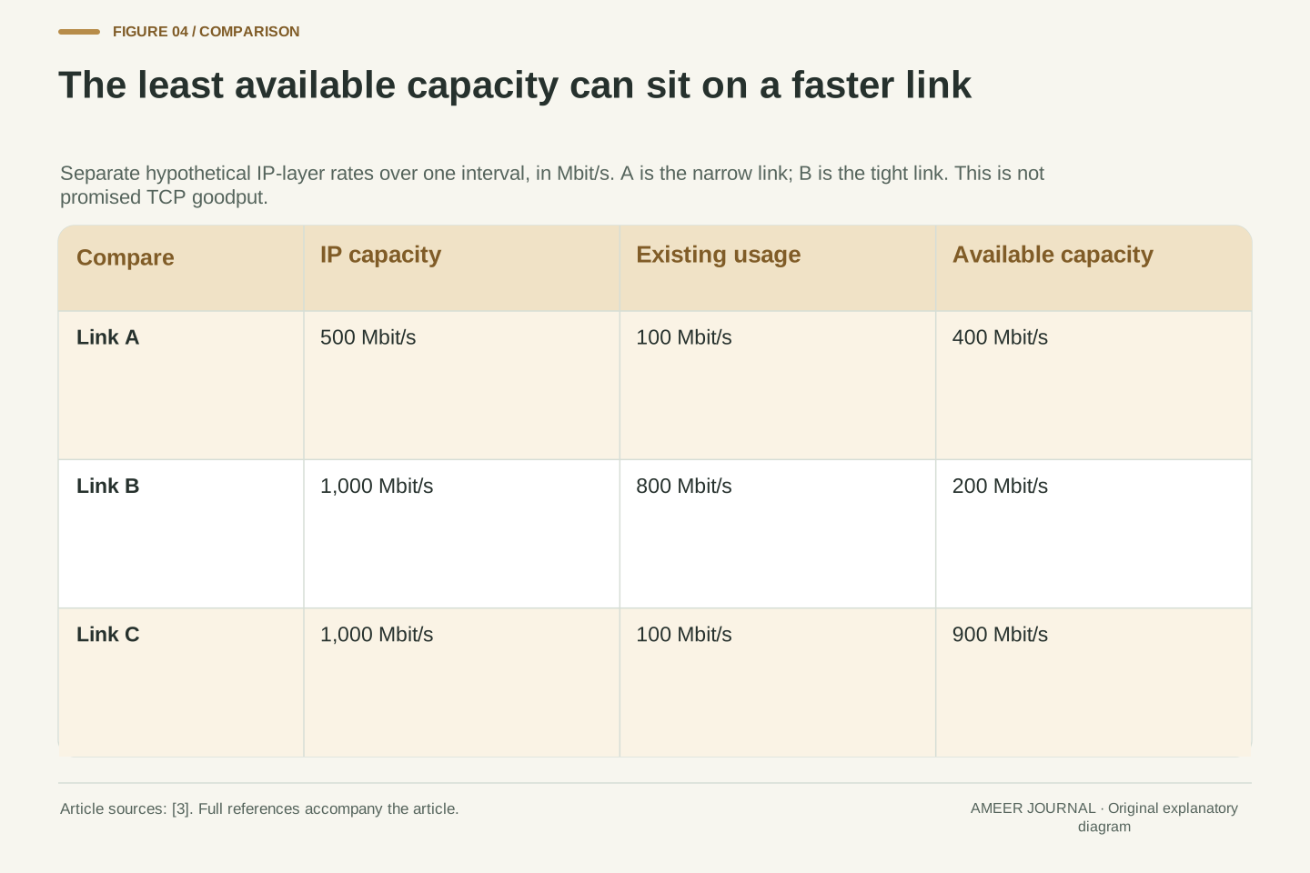
Here is a separate invented example, with every rate measured at the IP layer over the same interval. Link A has 500 Mb/s of capacity and 100 Mb/s already used, leaving 400. Link B has 1,000 Mb/s and 800 already used, leaving 200. Link C has 1,000 Mb/s and 100 already used, leaving 900. A has the smallest capacity, but B leaves the least room.

Under that model, the available path capacity is 200 Mb/s, set by B. Those numbers are IP-layer quantities, including IP headers; they are not the earlier nominal Ethernet labels or a promise of 200 Mb/s of file data. [3] The example explains why checking only the slowest advertised port can miss the active limitation. It also explains why a result from a quiet period may differ from one recorded while the same route carries other traffic.

RFC 5136 defines available link capacity as capacity multiplied by one minus utilization, equivalently capacity minus usage under its definitions. Available path capacity is the minimum corresponding available link capacity. It calls the minimum-capacity link narrow and the minimum-available-capacity link tight. [3] Both the layer and observation interval must remain consistent; these are not interchangeable labels for any slow-looking interface.

In a separate constructed IP-layer example, let capacities for links A, B and C be (500, 1,000, 1,000) Mbit/s. Existing usage over the same interval is (100, 800, 100) Mbit/s. Available capacities are therefore (400, 200, 900) Mbit/s. A is narrow, while B is tight; the available path value is 200 Mbit/s. The calculation uses stipulated average rates, not sampled switch counters.

This result is not a guaranteed allocation to a new TCP connection. It describes the chosen capacity model at the IP layer, whereas TCP behavior and unique application delivery require additional information. RFC 5136 explicitly separates transport-level bulk transfer capacity from these IP-layer definitions. [3] Traffic changes and short bursts can also make a different interval tell a different story, so the interval belongs with the result rather than disappearing from the report.

Imagine a transfer result that records 420,000,000 unique file bytes delivered in six seconds. Dividing gives 70,000,000 bytes per second, or 70 decimal MB/s. Multiplying by eight gives 560 Mb/s. The two rates describe the same constructed result. A capital B means bytes; a lower-case b means bits. Throughout this article, mega means one million, so no binary-unit conversion is hidden in the comparison.

The word “unique” also matters. If some data is transmitted again, those extra transmissions do not make the completed file larger. A traffic counter can count a different population from an application’s finished-file counter. RFC 5136 distinguishes unique transport data from IP-layer bits; RFC 6349 separately accounts for retransmitted bytes. Microsoft’s interface counters also include traffic such as broadcast and multicast, which may not belong to the particular file being copied. [2][3][4]

The six-second interval needs a definition too. Did it include connection setup and opening the file, or only the central transfer period? Did the interface counter cover other activity? The hypothetical 560 Mb/s result cannot answer those questions by itself. Preserve the source of the byte count and the start and finish events before comparing two displays or deciding how much of the link was useful to this job.

For a constructed application result, B = 420,000,000 unique file bytes and Δt = 6 s give B/Δt = 70,000,000 B/s = 70 MB/s, or 8B/Δt = 560 Mbit/s. Decimal units are used throughout. The numerator and denominator define the result; a link-rate field contains neither this file population nor these timing boundaries.

Counter semantics differ by layer and implementation. RFC 3635’s specified interface octet counters include MAC headers and FCS but exclude preamble and delimiter; RFC 5136’s IP bits include IP headers; its bulk-transfer discussion excludes headers and retransmitted duplicates from unique data. [1][3] Microsoft’s documented interface counters include multiple traffic classes, and RFC 6349 separately tracks retransmissions. [2][4] These examples explain why different counters can all be correct while producing different rates.

The interval can include setup, application waits and final processing, or it can isolate a sustained middle period. Neither convention is inherently the same experiment. The report should name the population, direction and timing events, and state whether unrelated traffic is included. Without those details, dividing one counter by a nominal link rate may produce a precise percentage that does not measure the file-transfer efficiency the reader intended.

A complete file copy has to supply data at one end and consume it at the other. Imagine a sender that can provide only 50 MB of useful file data each second. Even a path with room for more cannot deliver that particular file faster than it is supplied in this steady example. A receiver that processes incoming data slowly can create another limit. The connection label describes neither application’s work rate.

The testing framework in RFC 6349 requires the endpoint to be capable of generating and receiving the traffic being assessed. It also asks reports to identify the TCP implementation and test conditions. [4] A memory-based traffic result and an application copying a stored project may therefore answer different questions. The latter includes its data source, protocol processing and destination workflow, while the former can intentionally examine a narrower path.

When a good network result sits beside a slower file operation, identify the work included in each result. The difference alone does not identify a cable, disk or processor fault. Our 50 MB/s source limit explains one possible boundary. A useful bottleneck claim names the constrained stage and the observations supporting that conclusion.

Application goodput depends on a complete pipeline. In a separate steady hypothetical case, a sender supplies unique file data at 50 MB/s, or 400 Mbit/s. A path with a higher payload ceiling cannot make this application supply bytes faster. Receiver processing, data preparation and other endpoint work can impose additional constraints. These are rate-balance observations, not a benchmark of a particular storage device or processor.

RFC 6349 requires test hosts to support the intended stateful TCP workload and calls for identifying the implementation and relevant conditions. [4] Its historical hardware recommendations are not used as claims about present equipment. The enduring point is workload capability: a generator that avoids file-system work and an application that reads, processes and writes a project can exercise different resource sets.

TCP offers an application byte stream, not a guarantee about the time needed for every surrounding application operation. [5] A comparison should state whether it times transport delivery, completion of a file API operation or some further validation. When those boundaries differ, the difference between results is not automatically attributable to the Ethernet segment. Evidence that isolates a stage is needed before replacing a broad observation with a specific causal explanation.

A reliable transfer does not treat an unlimited amount of unacknowledged data as safe to send. TCP has a receive window reflecting what the receiver can accept, and congestion control also limits sending. The amount allowed to remain in flight can change during a connection. Round-trip time measures the trip involved in sending data and receiving a response. These transport conditions are separate from the Ethernet link rate. [4][5]

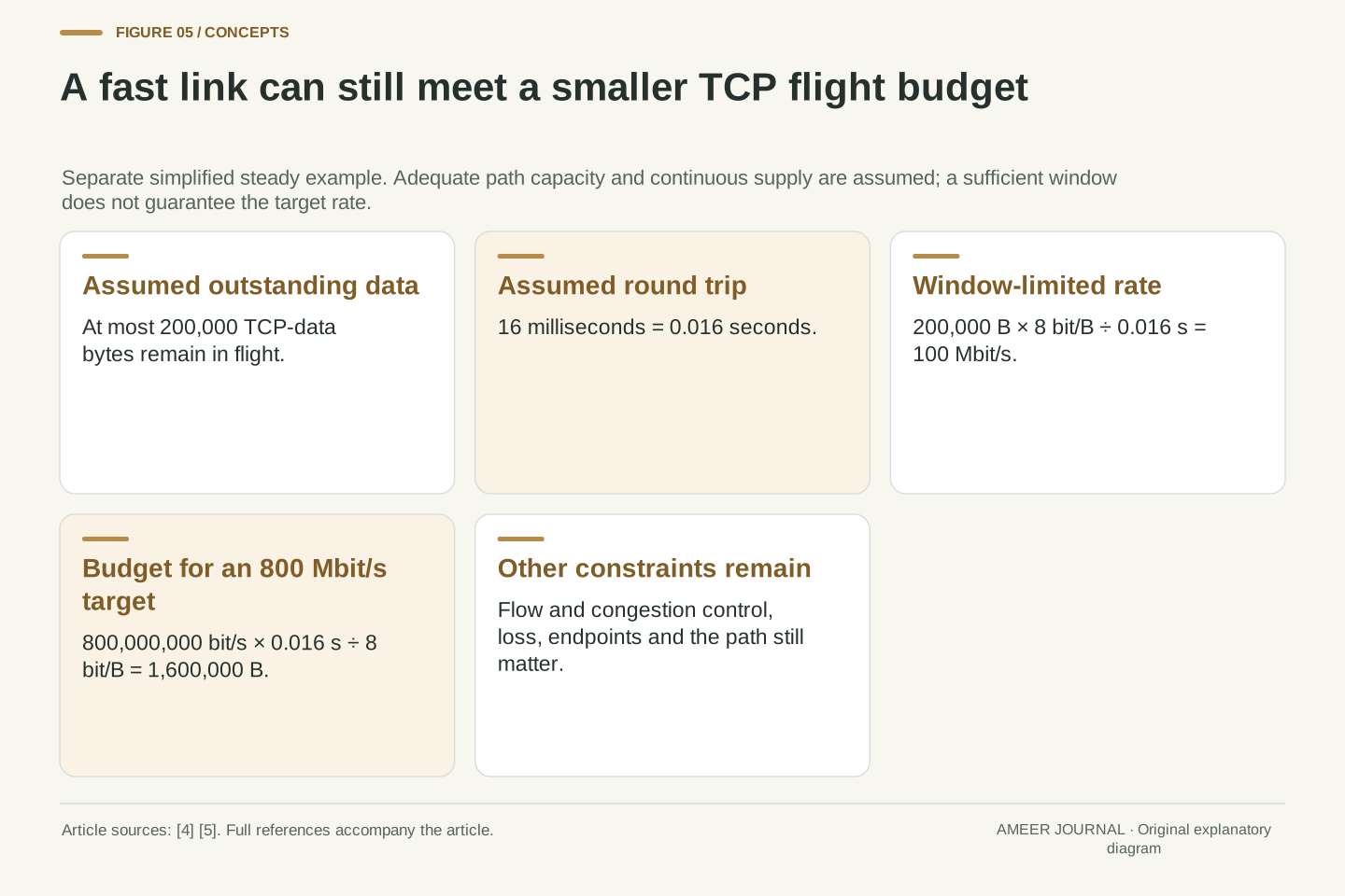
In another simplified example, assume at most 200,000 TCP-data bytes can remain in flight and the round-trip time is 16 milliseconds. Replacing that amount once per round trip gives 200,000 × 8 ÷ 0.016 = 100,000,000 bits per second, or 100 Mb/s. A gigabit local connection does not by itself remove that limit. The example assumes steady progress and enough capacity elsewhere to isolate the window relationship.

To sustain 800 Mb/s at that same 16-millisecond round trip, the corresponding flight budget would be 1,600,000 bytes. Having that budget would not guarantee the rate: the path, congestion control and endpoints still matter. RFC 6349 explains this relationship between flight capacity and delay, while RFC 9293 allows different conforming congestion-control algorithms. [4][5] The calculation helps interpret a result; it does not select a buffer setting for an unknown network.

Outstanding TCP data is constrained by receiver flow control and sender congestion control. RFC 6349 discusses the minimum of advertised receive and congestion windows, with send-buffer capacity also relevant; RFC 9293 keeps congestion-control algorithms distinct from the base transport specification. [4][5] A nominal link rate therefore does not determine a connection’s usable flight budget.

For a simplified steady window-limited model, take W = 200,000 data bytes and RTT = 0.016 s. The rate bound 8W/RTT is 100 Mbit/s, assuming continuous application supply and no tighter constraint. Conversely, a target TCP-payload rate of 800 Mbit/s at this RTT corresponds to R × RTT/8 = 1,600,000 bytes in flight. These are original inputs to the documented bandwidth-delay relationship. [4]

The flight budget is necessary within this model, not sufficient evidence that the target will be achieved. Window variation, acknowledgment behavior, congestion, loss and endpoint limits can change the outcome. [4][5] A transfer-start interval also differs from an established steady regime. The numerical example is deliberately separate from the earlier busy IP-path case; its 800 Mbit/s target is not being assigned to that path’s 200 Mbit/s available-capacity model.

Suppose one result reports several simultaneous transfers added together, while another reports one file. A larger total does not show that the single file could have reached the same rate. Similarly, uploading to one endpoint and downloading from another changes both the direction and the work being timed. Keep the number of connections, sender, receiver and direction with the reported result rather than treating every speed display as the same test.

The protocol frameworks attach results to their layer, interval, path and transport conditions. RFC 6349 also distinguishes measured results from an ideal achievable value and records effects such as retransmission and increased round-trip delay. [3][4] Two similar average data rates can therefore hide different behavior. One may involve stable delivery; another may combine bursts and waits. An average alone cannot describe every pause that an interactive application experiences.

Start with existing observations: the active interface, its operational state, the endpoints, counted bytes and timing scope. Ask which additional observation would distinguish the competing explanations. A precise display can be correct while answering a different question from the one you had in mind. Matching that question makes the comparison useful.

Aggregate throughput across connections and goodput for one connection are different observables. Parallel streams can exercise different transport windows or resource allocations; their sum does not establish the achievable rate of one stream. Endpoint selection, direction and local-versus-remote routing also affect the interpretation. RFC 6349’s framework explicitly includes single and multiple connection conditions rather than treating them as one interchangeable result. [4]

Match the layer, packet population, interval and transport assumptions before comparing percentages. RFC 5136 makes time and interval part of its definitions, and RFC 6349 distinguishes transfer time, retransmission efficiency and buffer-related delay. [3][4] Similar average goodput can coexist with different latency or loss behavior. Conversely, an average difference may result from a changed endpoint workload rather than a changed local Ethernet rate.

For an explanatory record, retain the evidence already available and state the unresolved alternatives. A counter difference may require a population check; a local-versus-remote difference may require path information; a single-versus-parallel result may require flow-level context. These are diagnostic questions, not a prescription to saturate a live network or alter transport settings. The aim is to make the next inference narrower and testable instead of attaching a generic fault label to an aggregate number.

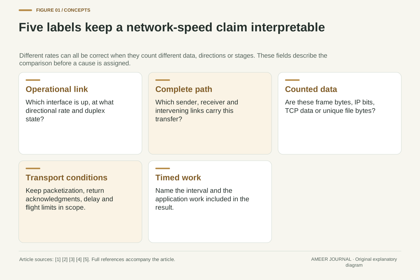
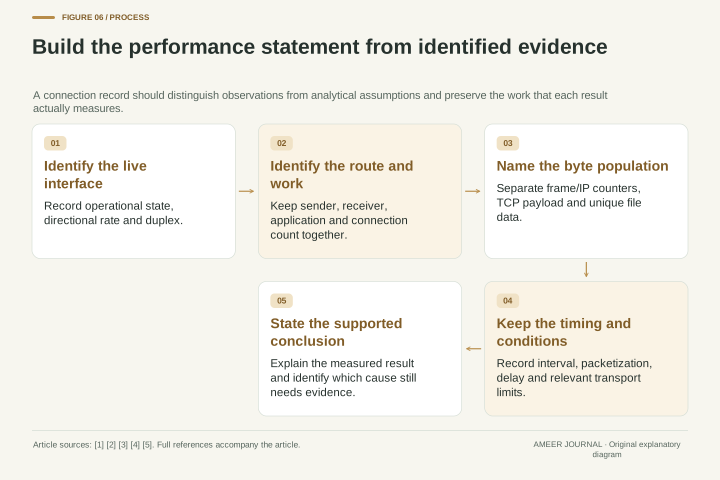
A useful record has five parts: the established local link and direction; the sender, receiver and path; the packet and header assumptions; the transport conditions; and the application’s byte count with its timing interval. These fields turn “my gigabit connection is slow” into a statement someone can investigate. They also separate facts you observed from assumptions used in an estimate.

For example, the constructed 420 MB transfer in six seconds supports “70 decimal MB/s of unique file data during this interval.” It does not independently prove a cable fault, a 560 Mb/s link, or the amount of available IP capacity. The 949.3 Mb/s calculation answers a different question under the full-packet model. RFC 5136’s layer definitions and the TCP testing framework explain why both numbers need their boundaries. [3][4]

The connection label identifies one capability and can help locate an unexpectedly slow segment. Connect that local fact to the route, packet budget and completed job. A lower file rate then becomes a quantity you can interpret, with specific missing observations to investigate instead of an unexplained gap between two numbers.

A reconstructable report retains interface operational state, directional rate, complete endpoint/path identity, packetization, transport conditions and the application measurement definition. Configuration and capability fields should remain distinct from observed delivery. RFC 3635 and Microsoft provide concrete interface-reporting examples; RFC 5136 and RFC 6349 provide the layer and interval discipline needed to relate them to an end-to-end result. [1][2][3][4]

The original examples yield several compatible numbers: 1 Gb/s nominal directional rate, approximately 949.285 Mbit/s ideal TCP data under one framing model, 200 Mbit/s available IP capacity in a separate busy path, and 560 Mbit/s unique file data in a separate constructed transfer. They are not four measurements of one network. Each belongs to its stated inputs and accounting boundary.

A real explanation should make the same distinctions before connecting the values. Identify what is supported, what was measured and what remains assumed. The purpose of the packet and window calculations is to reveal which extra inputs an inference needs, not to manufacture a universal expected score. A local link rate is one useful fact; a complete performance claim also identifies the data, path and work to which its rate actually applies.