What you’ll take away
- Identify the channel or derived product before giving a satellite image a physical meaning.
- A repeated regional view and coverage built from orbital passes represent different observing patterns.
- Thermal imagery can operate at night, but its brightness temperatures are not automatically street-level air temperatures or rainfall.
- Use observation timestamps for calculations; animation speed is only a presentation setting.
- Feature motion, rainfall estimation and a local forecast require different evidence and assumptions.
A moving cloud picture is an observation to interpret
A satellite loop shows a bright cloud feature moving toward your town. Does that mean rain will reach your street in half an hour? The picture alone cannot settle that question. First you need to know what was measured, when it was measured and how the display was made. NOAA describes satellite products as measurements and derived information used by forecasters, rather than a single image that contains every part of a local forecast. [2]
Start with a more careful sentence: this product shows a particular feature at these observation times. You can then ask what the feature suggests, what other evidence is needed and whether an official forecast agrees. This keeps a useful observation from becoming a prediction merely because the animation looks convincing. The screen's smooth movement can make changes feel more continuous and certain than the underlying observations justify.
We will examine orbit, channel, timing and interpretation through invented examples. No real storm or local forecast was analyzed for this article. The examples are designed to help you read a satellite product and recognize which conclusions its evidence can support. The important distinction is between observing radiation, making a product from it, interpreting the atmosphere and predicting what happens next.
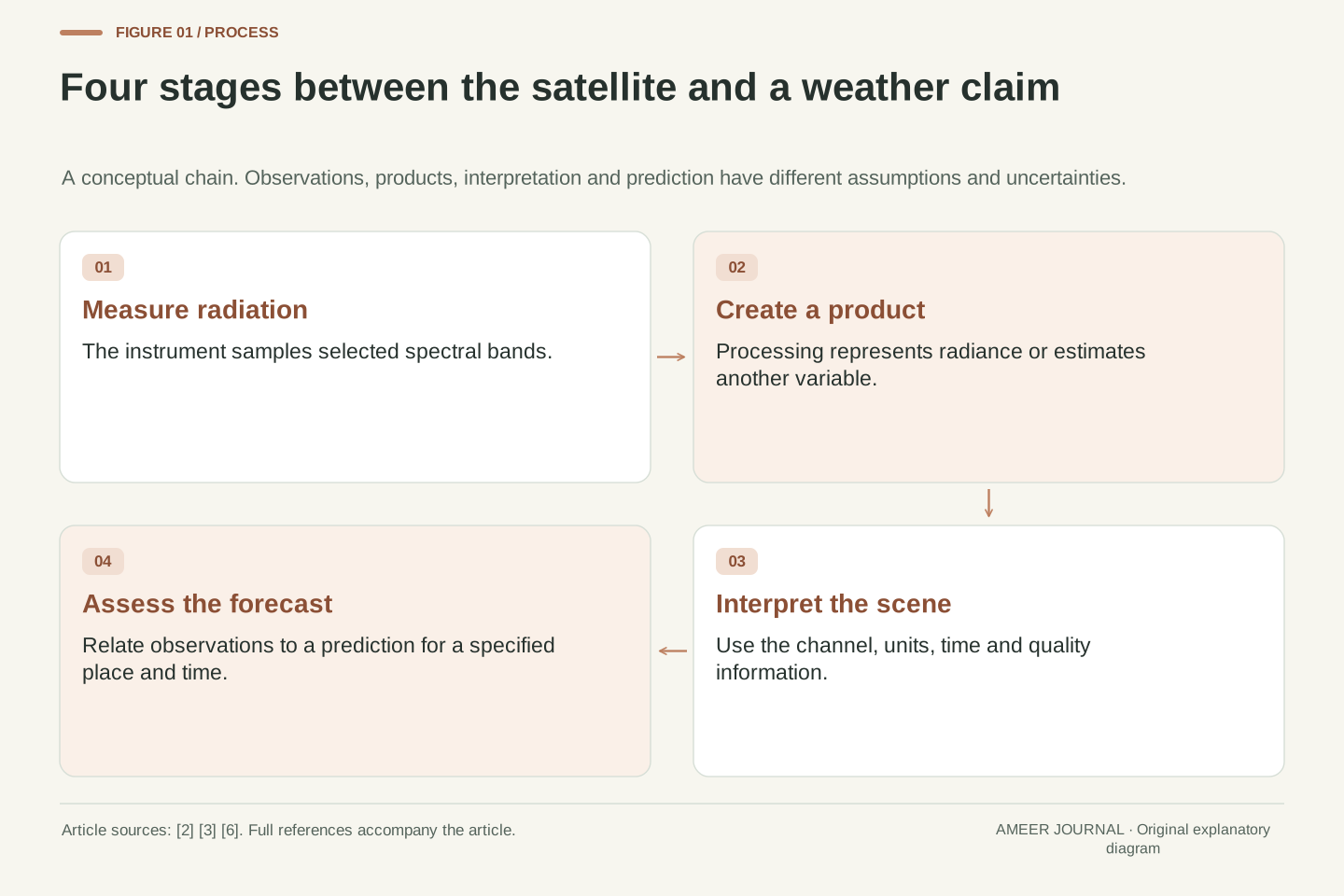
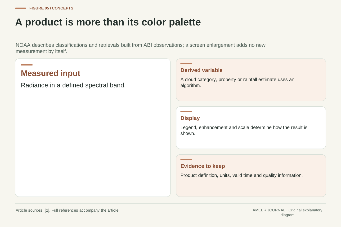
Satellite imagery is a representation of remotely sensed observations, with processing and display choices between the instrument and the viewer. NOAA's GOES-R product descriptions distinguish measured radiances from derived quantities such as cloud properties and estimated rainfall rates. [2] A colored image therefore does not carry a single universal meaning. Its interpretation depends on the instrument, spectral band, product algorithm and time metadata.
Separate an observation statement from an inference and a forecast. A feature at a stated location and observation time is evidence about the sampled scene. Interpreting that feature requires a physical model or product definition. Predicting its future location or associated surface weather adds further assumptions. The workflow can be valuable while uncertainty remains at each transition; a compelling animation does not eliminate those transitions.
The calculations below are explicitly hypothetical and are not a forecast demonstration, satellite validation study or analysis of an actual event. They isolate temporal sampling, feature tracking and the distinction between a measured signal and an inferred quantity. The objective is an auditable reading method: identify the product, preserve its units and timestamps, and limit the conclusion to what the observation and supporting evidence actually establish.
The orbit determines which view can be repeated
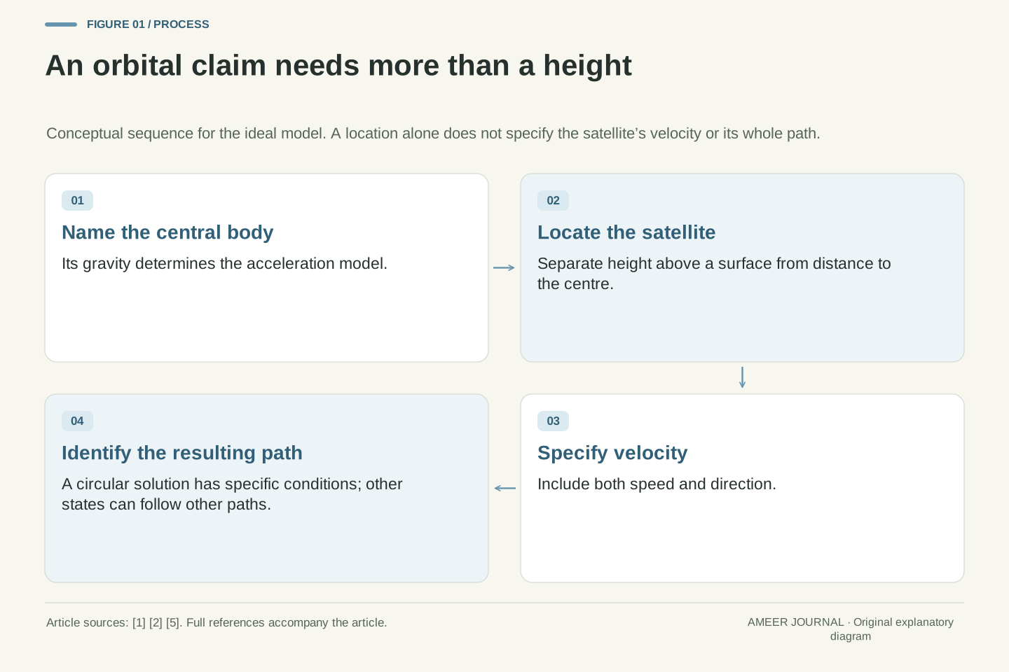
A geostationary satellite travels around Earth while appearing to remain above the same equatorial location. NASA explains the orbital conditions that make this possible and notes their usefulness for meteorological satellites. [1] The satellite is moving; its motion matches Earth's rotation. That arrangement gives an instrument a stable regional viewpoint from which it can repeatedly observe changing weather, subject to its actual scanning schedule.
A polar or near-polar satellite takes a different route. Earth turns beneath its orbit, allowing successive passes to sample different ground tracks. NASA describes this geometry in its orbital guide. [1] Broad coverage is built over time rather than obtained by seeing the entire surface at one instant. The revisit of your location depends on the actual orbit, instrument swath and observing arrangement.
These are complementary viewing patterns, not a rule that one type is best for every weather question. A repeated regional view can help show change; broader sequences of passes can supply observations elsewhere. A geostationary spacecraft also cannot see through Earth to the far side. Before comparing two products, check whether their pictures represent the same place and time, rather than assuming every satellite image is a simultaneous global snapshot.
An ideal geostationary orbit is circular, equatorial and prograde, with a period matching Earth's rotation relative to inertial space. Its apparent ground position is approximately fixed, maintained operationally within the mission's constraints. NASA distinguishes this case from the broader geosynchronous category and identifies meteorological use. [1] A stable viewing geometry supports repeated observations of a region, but it does not determine a particular instrument's scan cadence.
For a polar orbit, Earth rotates below the orbital plane, so successive passes provide different ground tracks. NASA describes this coverage geometry. [1] Near-polar meteorological missions use their specified orbits and instrument swaths; no universal daily revisit count follows from the word polar. Coverage over a time interval must be distinguished from simultaneous coverage, and a composite can contain observations acquired at different times.
Line-of-sight geometry also limits the visible region: a geostationary observer cannot see the opposite side of the solid Earth. This is a geometric constraint, not a temporary data outage. Compare orbit, field of regard, scan schedule and product assembly separately. The article makes no claim about which named spacecraft is currently serving a particular longitude, how many operational satellites exist or the availability of a live product today.
The instrument measures energy before the image has a meaning
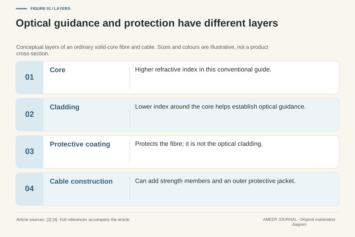
A weather imager is sensitive to selected parts of the electromagnetic spectrum. NOAA's atmospheric-window explanation shows why the choice matters: the atmosphere lets some wavelengths through more easily and absorbs others. [3] Different channels therefore offer different information. They are not interchangeable photographs with different decorative colors.
For the GOES-R Advanced Baseline Imager, NOAA describes measured radiation being converted into brightness values or brightness temperatures, then used to build other products. [2] A displayed temperature is therefore tied to that measurement and product. It is not automatically the temperature you would read from a thermometer outside your house. Keep the channel name and unit attached to the image whenever you describe it.
Imagine two maps of the same region, one showing reflected sunlight and another showing thermal radiation. Their contrast can differ even when neither map is wrong. They are answering different sensing questions. Before deciding that a feature suddenly appeared or disappeared, check whether you changed the measurement being displayed. A valid comparison needs a common meaning for the values as well as matching geography.
Radiance is the radiometric quantity underlying many satellite imaging products. Instrument channels sample specified spectral regions, and atmospheric transmission and absorption vary with wavelength. NOAA's atmospheric-window guide explains why channel selection changes the information available about the Earth-atmosphere system. [3] A channel is therefore part of the measurement definition, not merely a display style selected after an otherwise identical observation.
NOAA documents GOES-R ABI visible/infrared measurements being represented as brightness values and brightness temperatures and used by downstream algorithms. [2] A brightness-temperature image is a representation of band radiance, with interpretation governed by the channel and scene. It should not be silently relabeled as near-surface air temperature, cloud height or rainfall intensity. Those quantities require their own interpretation or retrieval product.
When comparing images, keep spectral identity, units, processing and valid time consistent. A change in contrast after switching channels is not necessarily a change in the atmosphere. This is an inference about measurement comparability, not a claim that one channel perfectly isolates one physical layer. Treat the product definition as part of the evidence, and retain its limitations when explaining what a bright or dark feature represents.
A day-to-night display may change the observation type
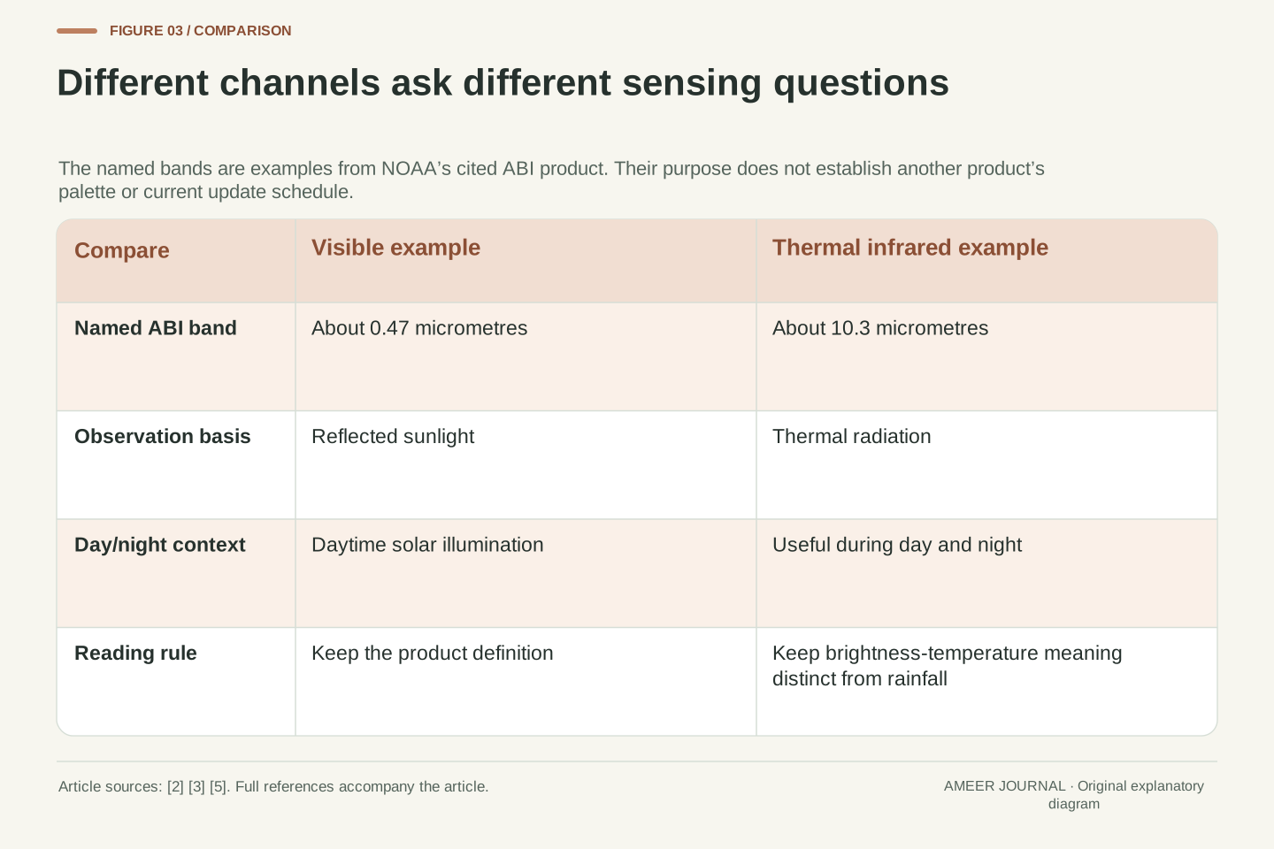
Visible imagery commonly relies on reflected sunlight. A thermal infrared window channel can provide information during both day and night. NOAA's combined-imagery page illustrates the distinction with an ABI visible band near 0.47 micrometres and a thermal infrared band near 10.3 micrometres. [5] Those are named examples, not a statement that every channel containing the word infrared behaves identically.
This matters when a website changes its displayed layer after sunset. A bright feature in the daytime portion and a bright feature at night may be bright for different physical reasons. Check the product legend and description before treating the whole sequence as a single unchanged measurement. The display can be useful while still needing that explanation.
For a simple reading exercise, pause before and after the transition and record the layer names and observation times. Ask whether the feature you followed is represented by the same quantity in both frames. You do not need to calculate a temperature to notice that the comparison changed. The first task is to identify what the display now means, then decide which comparisons remain valid.
Reflected-solar and thermal-emission imagery have different illumination dependence. NOAA's cited product uses the ABI 0.47 micrometre visible band for daytime observations and a 10.3 micrometre thermal infrared window band for day/night cloud information. [5] This is a scoped product example. It is not a universal statement about every visible/near-infrared/infrared channel or every multispectral composite.
A composite or day/night presentation can change its input channels while maintaining a familiar geographic display. Consequently, a visual continuity across the transition need not imply radiometric continuity. A feature's brightness or color may encode a different measured quantity. Before comparing pixel values or feature intensity, verify whether the layer, enhancement and processing definition remained the same.
A practical metadata check records the displayed product on each side of the transition, its unit, palette and valid time. This is an analysis procedure, not a report of a specific website's current implementation. If the product changes, compare physical interpretations supported by its documentation rather than treating identical screen colors as identical observations. Channel awareness prevents a display transition from being mistaken for sudden atmospheric evolution.
A cold-looking cloud top is not a rain gauge
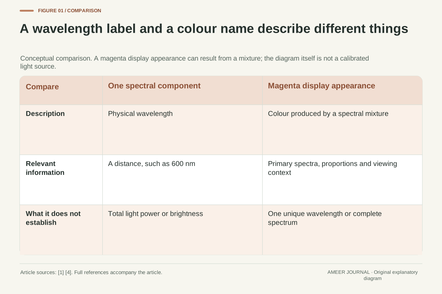
Infrared imagery can help reveal emitting temperatures associated with clouds or the surface. NOAA's Climate Prediction Center warns that cold signals do not always match precipitation: cold terrain can contribute, and a detected cloud need not be raining. [4] A color that suggests cold cloud tops therefore does not, on its own, tell you the amount of rain reaching your street.
There is a separate step when a product estimates rainfall. NOAA's GOES-R product description says its ABI rainfall-rate algorithm uses infrared brightness temperatures and is calibrated against microwave-derived rain rates. [2] That is an estimate produced through an algorithm and supporting information, not a direct reading of the ordinary cloud image as though every pixel were a rain gauge.
Suppose a fictional screenshot has an intense red patch. Before saying it means heavy rain, find out what red represents on that exact product. It could be a temperature enhancement rather than a rainfall scale. Read the legend, units and product name, then compare appropriate local weather information. The color becomes meaningful through its definition; it does not carry one fixed meteorological message across every map.
Thermal infrared information can indicate the temperature of emitting cloud or surface features, but the mapping from that signal to surface precipitation is not one-to-one. CPC's explanation expressly notes cold terrain and non-precipitating clouds as counterexamples to a simple cold-equals-rain inference. [4] The visual image does not directly supply rainfall at a ground location merely because low brightness temperatures are present.
NOAA describes the ABI rainfall-rate product as an algorithm using infrared brightness temperatures with calibration against microwave-derived rain rates. [2] That additional processing creates a distinct estimated variable. Preserve the difference between the input observation, the retrieval algorithm and the resulting precipitation estimate. A product label or color table alone does not turn an indirect estimate into an in-situ measurement.
For a hypothetical red patch, first inspect whether the legend is expressed in temperature, precipitation rate or a qualitative composite scale. Do not transfer the meaning of red from another product. A claim about ground rainfall requires evidence and an appropriate product definition at that boundary. The distinction is methodological: the article does not assert the presence, amount or future timing of rain in an actual location.
Read observation time before animation speed
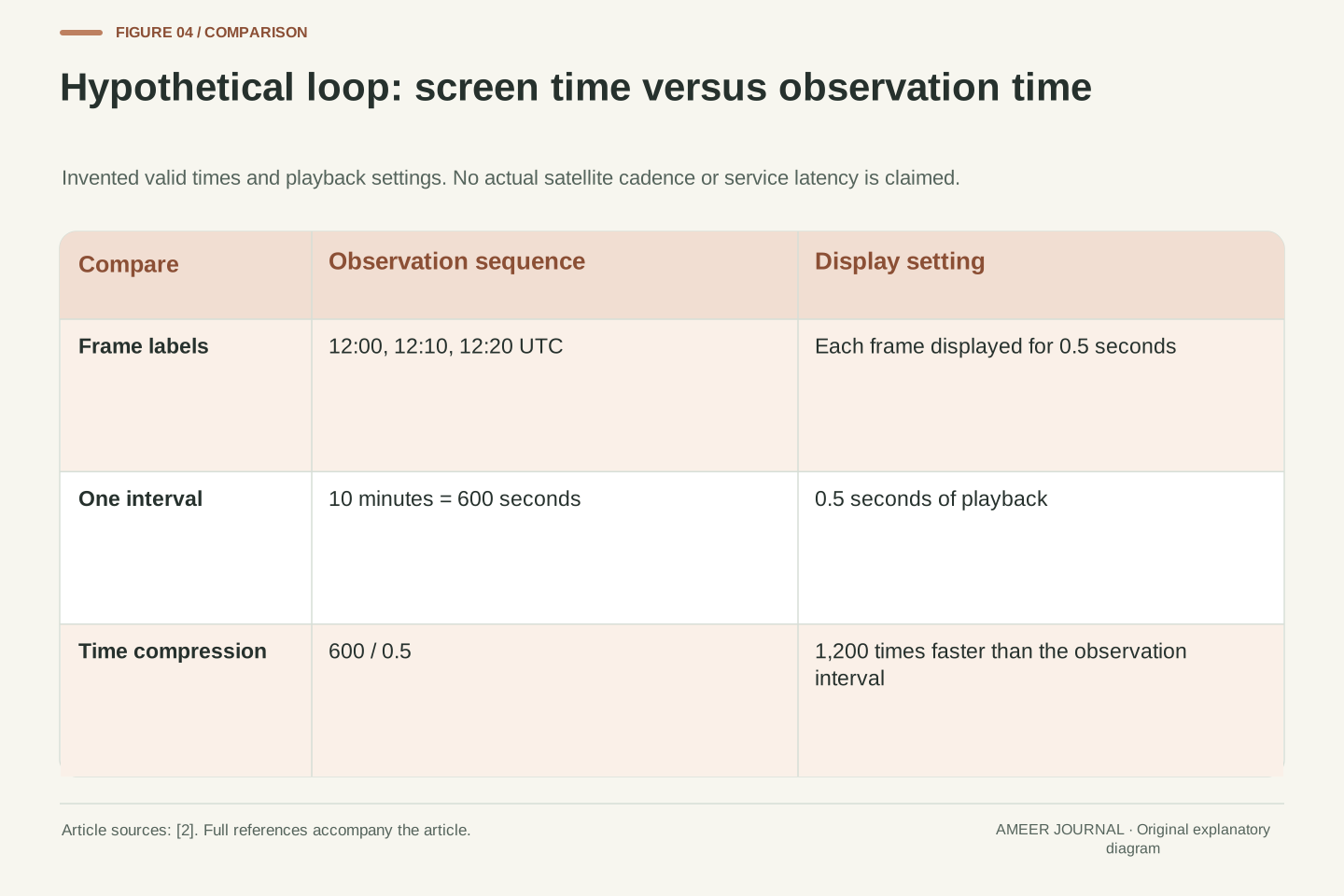
A fast animation is not fast-moving weather. Imagine three frames labeled 12:00, 12:10 and 12:20 UTC, with each frame shown for half a second. The observation interval is ten minutes even though the screen advances almost immediately. One ten-minute step compressed into half a second represents a playback factor of 1,200. These are invented display settings, not the update schedule of a satellite service.
Check the timestamp on each frame instead of assuming every step is equally spaced. Missing frames or a changed selection could alter the interval. Also separate the observation time from the time the page was opened or the image was delivered. Those labels answer different questions. An attractive loop can still show an older scene than a viewer expects if the time information is ignored.
For a comparison you want to repeat, record the first and last observation times, the time zone and the number of usable intervals. If a timestamp's meaning is unclear, keep that uncertainty in the description. Saying a feature changed between two named observations is more useful than saying it changed quickly because the animation played quickly.
Define observation time separately from playback time. In a constructed sequence with valid times 12:00, 12:10 and 12:20 UTC, adjacent observations are 600 seconds apart. Displaying each frame for 0.5 seconds gives a temporal playback factor of 600/0.5 = 1,200 for each step. This is exact arithmetic for an invented presentation, not evidence about an operational scan mode or data latency.
A rate estimate must use acquisition or product-valid times with a clear interpretation. Page refresh time, file publication time and animation dwell time are different quantities. Unequal gaps must be preserved rather than replaced by an assumed cadence. If a product combines observations, its time definition should be read from the metadata before a single timestamp is treated as simultaneous observation of every location.
An auditable record contains the product name, valid-time labels, time standard and interval used for each comparison. It also identifies missing information rather than assigning a plausible schedule. These proposed controls prevent a display convenience from entering a physical calculation as if it were an instrument measurement. They establish how to inspect timing, not the current refresh behavior of a named satellite website.
Follow a feature without promising where rain will go
Now use the same fictional ten-minute intervals. Assume the same identifiable cloud feature moves 12 kilometres during the first interval and 6 kilometres during the second. Its calculated average speeds are 72 and 36 kilometres per hour. We chose those distances; no real cloud was tracked. The example shows why an observation interval and a distance measurement must accompany any speed claim.
Suppose a point along the assumed path is another 18 kilometres ahead. Extending the latest speed unchanged gives thirty minutes to that point. Extending the earlier speed gives fifteen minutes. Those are conditional arithmetic results, not two competing weather forecasts. We have already seen the feature's apparent movement change, so neither constant-speed extension is established by the observations alone.
A changing cloud shape adds another question: are you following the same feature in every frame? Growth, fading or a different selected edge can change the apparent track. Even a sound cloud-motion estimate does not, by itself, give surface rainfall arrival. The task is to describe what was tracked and which assumptions enter the next step, instead of converting a moving patch into a precise local promise.
Let a hypothetical identified feature have displacements d1 = 12 km and d2 = 6 km over two successive ten-minute intervals. The interval averages are 12/(10/60) = 72 km/h and 6/(10/60) = 36 km/h. These are constructed feature-tracking values, not measured atmospheric wind or precipitation motion. The calculation assumes the chosen feature and map distances are consistently identified.
For a location 18 km farther along an assumed unchanged path, constant-speed extrapolation at 36 km/h yields 0.5 hours, while 72 km/h yields 0.25 hours. The difference exposes sensitivity to a chosen motion assumption. Neither result follows as a forecast without establishing persistence of the feature, motion and relevant weather relationship. The arithmetic remains valid while the prediction can be unjustified.
Identification is part of the observation model: an evolving edge, newly formed cloud or fading feature can undermine correspondence between frames. Geometric cloud tracking also cannot be silently converted into a ground-rainfall forecast; the observation/retrieval distinction discussed earlier still applies. [2][4] Report the measured or hypothetical displacement, interval and assumptions separately from any operational forecast, preserving the possibility that the feature changes before reaching the extrapolated point.
A processed product needs its own definition
Weather services turn satellite measurements into many useful products. NOAA describes cloud masks, cloud-top properties and other information derived from the ABI observations. Its cloud mask can distinguish categories such as cloudy, probably cloudy, clear and probably clear. [2] Those labels show that interpretation can involve uncertainty rather than a perfectly sharp division between known cloud and known clear sky.
The display adds another layer. Colors and contrast make patterns easier to see, but their meaning belongs to the chosen palette and variable. A larger view on a screen also does not create an extra measurement. Zooming can help inspect what is available; it cannot establish fine detail that the source data never resolved. Treat display scale as a viewing choice, not evidence of a new observing capability.
When sharing an image, keep its product name, legend and timestamp with it. If you crop out the legend or replace the caption with a dramatic claim, the reader may lose the information needed to interpret the colors. A useful caption says what the product represents and what is inferred from it, especially when a derived category or estimate is being presented as a visual map.
Retrieval and classification products apply additional algorithms to the observations. NOAA's GOES-R documentation describes cloud masks with confidence-related categories and cloud-top height, temperature and pressure retrievals. [2] A labeled pixel is consequently an output of a specified method, not a guarantee that a complex atmospheric column has been measured without ambiguity. Product quality and validity belong to the interpretation.
Display processing is another transformation. Color enhancement or resampling can improve readability but does not by itself add independent radiometric observations. If a raster is shown at a larger screen scale, additional display pixels need not represent additional measured information. This is a statement about data representation, not an assertion of a particular instrument's native resolution or the processing used by a live service.
A reproducible interpretation preserves variable, unit, palette, product version where available, valid time and quality information. Distinguish an algorithmic category from the viewer's own inference. When an image is cropped for publication, retain enough metadata to reconstruct its meaning. Without those controls, a polished graphic can appear more certain or more finely measured than the underlying product definition supports.
Forecasting uses the observations through another model
Satellite observations help forecasting, but a forecast involves more than sliding cloud shapes across a screen. NOAA says the GOES-R spectral observations are used in numerical weather prediction, as well as in derived imagery products. [2] A model supplies a structured way to relate observations to an atmospheric state and its evolution. The image you see is one useful view of the evidence, not the complete forecast process.
NOAA's radiance-assimilation monitoring description shows another important distinction. It compares observed radiation with radiation simulated from a forecast model, and discusses contributions from observation errors, the atmospheric profile and the radiation calculation itself. [6] A disagreement therefore does not have only one possible cause. It would be too simple to declare either the satellite or the forecast wrong from the difference alone.
For everyday use, let the satellite loop help you understand the broad pattern and recent change, then consult the relevant forecast or warning for the local decision. Keep issue time and valid time in view. This does not make imagery less valuable. It gives each piece of information a clear role and avoids asking a picture to answer a question that requires additional analysis.
Numerical prediction and visual image interpretation are related but different uses of satellite data. NOAA documents radiances being used in weather prediction models as well as downstream image products. [2] Data assimilation connects observations with a modeled atmospheric state through observation and error treatment; prediction then evaluates the state's subsequent evolution. A visual extrapolation of one cloud feature does not reproduce that entire process.
NCEP's radiance-monitoring introduction discusses observed-minus-simulated radiance departures and bias correction. It identifies observation error, errors in the model-derived atmospheric profile and errors in the radiative-transfer calculation as contributors to those departures. [6] The simulated observable is important: the comparison must relate compatible quantities rather than subtracting an image color from a forecast temperature with a different physical meaning.
A departure therefore needs diagnosis, not an automatic attribution to one component. Likewise, an analysis or assimilation step is not a guarantee of forecast correctness. The useful conclusion is that imagery, retrieved products and numerical prediction occupy different stages of an evidence chain. When evaluating a forecast claim, specify the variable, location, valid time and verification evidence rather than treating an impressive satellite animation as a complete validation.
A short routine for the next satellite image
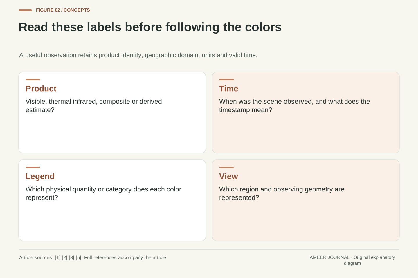
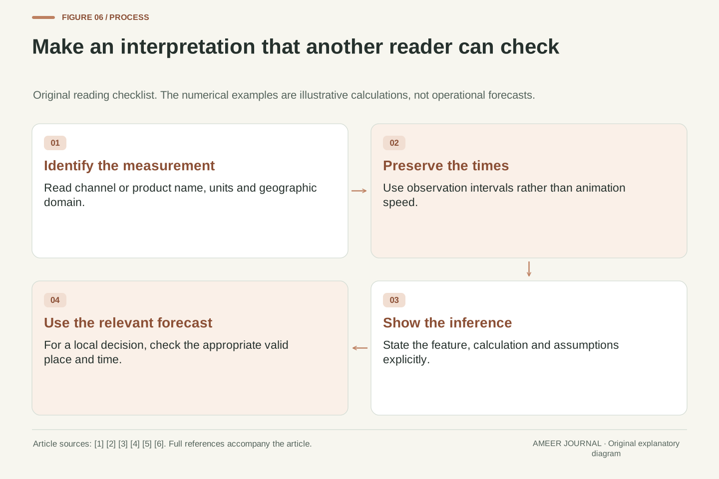
Before interpreting a satellite image, read its name and legend. Identify whether it shows reflected sunlight, thermal radiation, a combined display or a derived product. Check the observation time and region. Then state one observation in plain language, such as a feature changing between two named frames, without immediately adding a rainfall amount or arrival time that the image has not established.
If you calculate movement, preserve the distance estimate, the actual time gap and the feature you followed. If you compare colors, preserve the channel and scale. If you compare products from different orbits, check when each observed the place. NASA's orbit descriptions and NOAA's channel/product documentation explain why these conditions matter. [1][2][3][5] The reading routine connects those facts to an ordinary browser view.
Finally, label the step from observation to inference. Our invented feature moved at two different average speeds, and two simple extensions produced different arrival times; neither was a local forecast. A real decision deserves the appropriate current forecast or warning, with its own location and valid time. The satellite image helps you see the evidence more clearly when its limits and meaning stay attached.
Use a compact interpretation record: platform or product source, spectral/product identity, units, spatial domain, valid times, quality information and the precise statement being tested. Separate the acquisition geometry from product generation and presentation. NASA's orbit primer and NOAA's atmospheric-window, ABI and visible/infrared descriptions support those distinctions without providing a universal update schedule or local weather result. [1][2][3][5]
For a quantitative claim, retain the calculation inputs and their origin. A rate needs displacement and elapsed observation time; a temperature interpretation needs the proper band and radiometric meaning; a precipitation statement needs a suitable estimate or other evidence at that boundary. [2][4] Do not replace missing metadata with the playback speed, an assumed palette convention or a number borrowed from another sensor.
The hypothetical examples establish limited results: ten minutes per half-second display step is 1,200-times playback; 12 km and 6 km per ten minutes are 72 and 36 km/h; an 18 km continuation gives fifteen or thirty minutes only under the chosen constant-speed assumptions. Those calculations teach interpretation, not tomorrow's weather. Keep source scope and uncertainty visible when new products or observing systems are introduced, and update operational details only after checking the applicable documentation.
Sources & further reading
Explore the references behind this guide. External pages may change after our review.
- Chapter 5: Planetary Orbits - NASA ScienceNASA Science · Accessed 6 Nov 2026
- GOES-R Series Data Products | NESDIS | National Environmental Satellite, Data, and Information ServiceNOAA / NESDIS · Accessed 6 Nov 2026
- The Atmospheric Window | National Oceanic and Atmospheric AdministrationNOAA / National Weather Service · Accessed 6 Nov 2026
- IR Imagery InformationNOAA / Climate Prediction Center · Accessed 6 Nov 2026
- Visible & Infrared Imagery | NESDIS | National Environmental Satellite, Data, and Information ServiceNOAA / NESDIS · Accessed 6 Nov 2026
- Radiance assimilation monitoring: introductionNOAA / NCEP Environmental Modeling Center · Accessed 6 Nov 2026
Article updated 6 Nov 2026.
Found something we should revisit?
Good explanations get better with thoughtful feedback.