What you’ll take away
- Area-normalized resistance in m²K/W differs from complete-component resistance in K/W.
- Add equal-area layers within each complete path before combining independent parallel paths.
- For the stated parallel model, average area-weighted transmittances and then take the reciprocal.
- The original arithmetic R average of 4.2 overstates the correct effective R of 3.75 by 12 percent.
- Changing a branch or adding a connection requires preserving the network assumptions when recomputing its equivalent.
Two correct path ratings can produce one incorrect wall rating
An imaginary wall has a large region with an R-value of 4.5 and a smaller region with an R-value of 1.5. The large region occupies 90 percent of the wall. Would multiplying each value by its share of the area, then adding, give the wall's effective R-value? That tempting calculation gives 4.2. Under the particular heat-flow model developed here, the correct answer is 3.75. Both calculations use the same starting numbers; the difference is what gets averaged.
R describes resistance to heat flow. An easier path carries more heat for a given area and temperature difference, so the low-resistance region cannot be accounted for simply by averaging resistance labels. MIT's thermal-circuit explanation distinguishes adding layers along one path from adding heat flow through parallel paths [2]. We will apply that distinction to one fully specified wall model, including the units. The numerical wall is invented, not a tested product or a building design. PNNL's discussion of heat travelling through framing provides the real-world reason that more than one path can matter [3].
Consider a two-region wall whose complete path resistances, normalized by their respective areas, are 4.5 and 1.5 m²K/W. Their area fractions are 0.9 and 0.1. A direct weighted arithmetic mean gives 4.2 m²K/W. An independent parallel-path calculation instead gives an effective area-normalized resistance of 3.75 m²K/W. The discrepancy is an aggregation issue, not a change in the assigned material values.
The underlying balance adds heat-transfer rates between common temperature boundaries. Because each path's rate is proportional to the reciprocal of its resistance, averaging the resistances themselves does not preserve that balance. MIT presents the corresponding series and parallel thermal circuits [2]; PNNL identifies framing as a potential heat-transfer route through an insulated wall [3]. Here the geometry, values and outcomes are an original mathematical construction. The purpose is to distinguish an area-weighted conductance from an area-weighted resistance, identify the quantities that may be combined, and make the assumptions behind the resulting equivalent value visible.
Decide whether R belongs to a unit area or a complete component
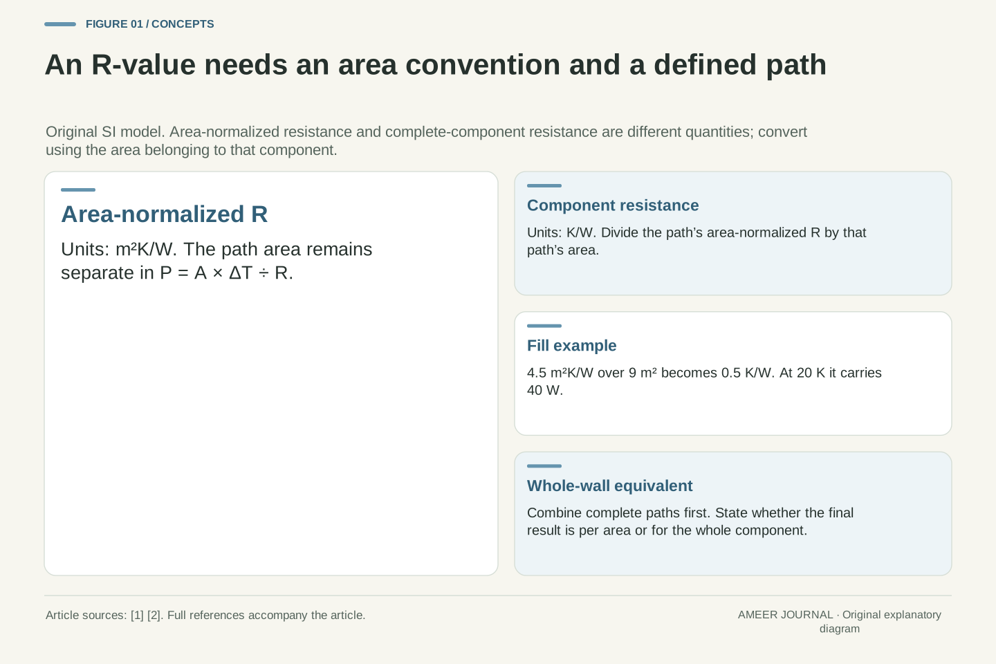
In this article every ordinary R-value uses SI units: square metres times kelvins per watt, written m²K/W. This describes resistance with area accounted for separately. OpenStax defines the slab's R factor from its thickness divided by its thermal conductivity, and distinguishes this convention from the customary units used on some insulation labels [1]. A bare number from another unit system cannot be dropped into our calculations unchanged.
For one uniform path, multiply its area by the temperature difference and divide by its R-value to find the assumed steady heat-transfer rate. A path covering 9 m² with R = 4.5 m²K/W and a 20 K difference therefore carries 9 × 20 ÷ 4.5 = 40 watts. The same material arrangement over a different area would carry a different total rate.
A complete component can instead be assigned a resistance measured in K/W. Divide its area-normalized R by its area: this 9 m² component has 4.5 ÷ 9 = 0.5 K/W. Dividing the 20 K difference by 0.5 K/W gives the same 40 watts. The two conventions agree when the area is handled consistently.
Use R for area-normalized resistance in m²K/W. For a uniform slab of thickness d and conductivity k, R = d/k. The finite component resistance is R_th = d/(kA) = R/A, with units K/W. OpenStax's area-normalized formulation and MIT's component-resistance formulation use the same physics but assign different meanings to the letter R [1][2]. We keep the area convention explicit rather than transferring a symbol uncritically between them.
With P denoting heat-transfer rate, the equivalent expressions are P = AΔT/R and P = ΔT/R_th. For A = 9 m², R = 4.5 m²K/W and ΔT = 20 K, the component resistance is 0.5 K/W and P = 40 W. A temperature difference of 20 K is also a difference of 20 Celsius degrees; no absolute temperature is needed for this constant-property calculation.
Changing the area does not change the stipulated area-normalized R of that uniform arrangement. It does change the component resistance and total heat rate. Accordingly, a whole-wall K/W result must be converted using the whole-wall area before comparing it with an area-normalized value. Customary US insulation units are outside this numerical example.
Add the layers within each path before combining the regions
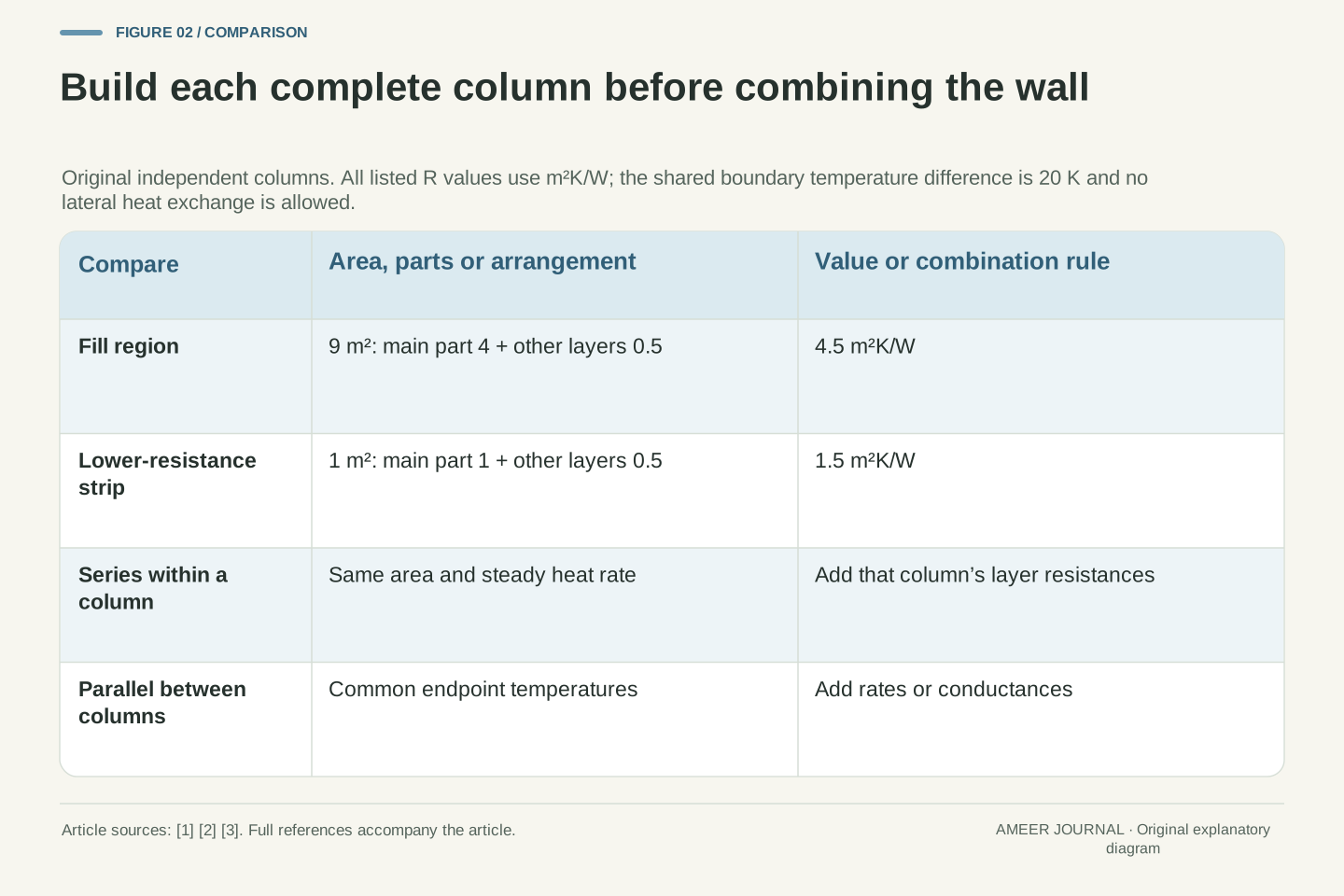
The two full-path values did not come from a single material alone. In the large region, assign the main insulating part R = 4 and the other layers together R = 0.5. Along the smaller region, assign a lower-resistance part R = 1 and the same other-layer contribution of 0.5. Every one of these numbers is in m²K/W. Following each path from one chosen boundary to the other gives totals of 4.5 and 1.5.
These additions are valid for the model because successive layers in one column have the same cross-sectional area and carry the same steady heat flow. Their temperature differences add along that route. OpenStax and MIT explain this series arrangement [1][2]. The full temperature difference is not applied independently across every layer and then counted repeatedly.
Keep the two columns separate at this stage. The smaller path does not acquire the large region's R = 4 merely because they share a wall drawing. Similarly, the 0.5 contribution belongs inside each complete path. Writing the paths out first makes it harder to mix a material-only rating with a rating that already includes its surrounding layers.
Construct each complete column as a series combination with a constant cross-sectional area. The fill column contains an assigned main-layer resistance of 4 and an additional series contribution of 0.5 m²K/W; the strip column contains 1 plus 0.5 m²K/W. Thus R_f = 4.5 and R_b = 1.5 m²K/W. The common numerical contribution means the same area-normalized resistance occurs within both paths, not that it is a single lumped element outside the parallel network.
For a steady equal-area column with no internal accumulation or side exchange, the rate P is common to its series elements. Each drop is ΔT_j = PR_j/A, so summing the drops yields ΔT = PΣR_j/A. The area-normalized series resistances therefore add under this arrangement [1][2]. Applying the full boundary difference separately across every series element would describe a different circuit.
The two columns may have different intermediate temperatures. Only their endpoint temperatures are stipulated equal. That distinction becomes important when considering whether lateral heat exchange is allowed. At this point, retain the complete path definitions and do not substitute the fill material's resistance for either the strip path or the complete wall.
Calculate each region’s rate with its own area
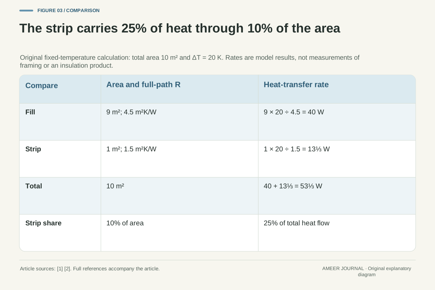
Give the entire wall an area of 10 m². The large fill region occupies 9 m² and the smaller strip occupies 1 m². Both complete paths connect the same two temperature boundaries, separated by 20 K. We assume steady conditions and no heat moving sideways between the columns. The strip is simply an assigned easier path; its numbers are not measurements of wood, steel or another building material.
The fill rate is 9 × 20 ÷ 4.5 = 40 W. The strip rate is 1 × 20 ÷ 1.5 = 13⅓ W. Add the rates because they are separate complete paths between the same boundaries: the wall carries 53⅓ W. This is the parallel-path accounting described by MIT [2]. Decimal versions of these exact fractions will be rounded when needed.
Notice that the strip occupies one tenth of the area but carries one quarter of the total heat flow. Area share and flow share are different quantities. The calculation has not made the small region physically larger; it has recognized that each square metre of that region offers less resistance.
Set total area A = 10 m², fill fraction f = 0.9 and strip fraction 1−f = 0.1. Then A_f = 9 m² and A_b = 1 m². Impose the same ΔT = 20 K across both complete paths. The independent-column assumption excludes lateral transfer and accumulation, allowing the component rates to be calculated separately and summed [2]. These values define the example rather than estimate actual framing performance.
The fill component has R_th,f = 4.5/9 = 0.5 K/W, while the strip has R_th,b = 1.5/1 = 1.5 K/W. Their rates are P_f = 20/0.5 = 40 W and P_b = 20/1.5 = 40/3 W. Therefore P_total = 160/3 W, approximately 53.333 W. A smaller area can have lower area-normalized resistance yet higher component resistance; the area conversion explains that apparent reversal.
The strip's flow fraction is (40/3)/(160/3) = 1/4, despite an area fraction of 1/10. This ratio concerns the stated parallel model and fixed boundary difference. It does not assign a universal flow share to framing or a particular material.
Average conductance first, then take its reciprocal
The effective R-value should describe one imaginary uniform wall that carries the same total rate over the same 10 m² and temperature difference. We already know that rate: 53⅓ W. Rearrange the single-path rule to calculate the required resistance: 10 × 20 ÷ 53⅓ = 3.75 m²K/W. This is why 3.75 is the useful equivalent value for the declared model.
You can reach it without first choosing the total area. Take the reciprocal of each complete-path R, multiply by that path's area fraction, and add. Here the result is 0.9 ÷ 4.5 + 0.1 ÷ 1.5 = 4/15. This quantity, commonly called U, measures heat-transfer rate per square metre per kelvin. Its units are W/(m²K). Taking its reciprocal gives 15/4, or 3.75 m²K/W [1][2].
The order of those steps matters. First translate each resistance into how readily its region carries heat, then combine those contributions. Only afterward turn the whole-wall result back into a resistance. This procedure preserves the rate we obtained by calculating the two regions separately.
Define the effective transmittance by P_total = AΔT U_eff. Substituting P_total = A_fΔT/R_f + A_bΔT/R_b and dividing by AΔT gives U_eff = f/R_f + (1−f)/R_b. This is an area-weighted mean of path transmittances, derived directly from the parallel rate balance [1][2]. Its units are W/(m²K).
The effective area-normalized resistance is R_eff = 1/U_eff, so it is the weighted harmonic mean of the positive full-path resistances. Numerically, U_eff = 0.9/4.5 + 0.1/1.5 = 1/5 + 1/15 = 4/15 W/(m²K). Hence R_eff = 15/4 = 3.75 m²K/W. The complete 10 m² wall has component resistance R_th,eff = R_eff/A = 3/8 K/W, which returns P_total = 20/(3/8) = 160/3 W.
These equivalent forms provide an internal consistency check. Summing branch rates, combining component conductances, and averaging area-normalized transmittances must agree when they describe the same endpoints, areas and independent paths. A disagreement indicates a changed assumption or a mismatched quantity.
Measure the error in the tempting arithmetic average
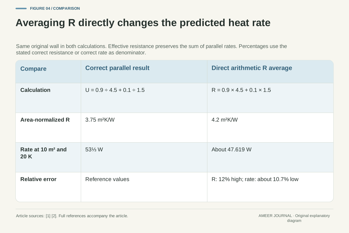
Now return to the tempting calculation: 0.9 × 4.5 + 0.1 × 1.5 = 4.2. That is a perfectly valid arithmetic average of the two listed resistance values. It is not the effective resistance that preserves the parallel heat flow. Putting 4.2 into the uniform-wall equation predicts 10 × 20 ÷ 4.2, or about 47.619 W, instead of the correct model result of about 53.333 W.
The resistance estimate is 0.45 higher than 3.75, which is a 12 percent overstatement relative to the correct resistance. The rate estimate is about 5.714 W lower than 53.333 W, which is approximately a 10.7 percent understatement relative to the correct rate. Those percentages differ because resistance and rate are reciprocally related, and each percentage uses its own reference quantity.
The arithmetic mean has given too much credit to the high-resistance area for this purpose. Heat is able to use both regions, and the easier region carries a larger share of the total than its area share alone suggests. The correction follows from the parallel balance, not from adding a mysterious penalty to the wall [2].
Let R_arith = fR_f + (1−f)R_b = 21/5 = 4.2 m²K/W. Substituting this into P = AΔT/R yields P_wrong = 200/(21/5) = 1000/21 W, approximately 47.619 W. The correctly aggregated model gives P_total = 160/3 W. The arithmetic average itself is mathematically defined; the error is treating it as the equivalent resistance of the specified network.
The resistance overstatement, using R_eff as denominator, is (R_arith−R_eff)/R_eff = (4.2−3.75)/3.75 = 3/25 = 12 percent. The corresponding rate understatement uses P_total as denominator: (P_total−P_wrong)/P_total = 3/28, approximately 10.714 percent. Reciprocal transformations do not preserve relative percentage differences. Reporting both as 12 percent would therefore introduce a second error after the averaging mistake.
The physical interpretation remains the conservation argument supplied by the thermal-circuit model [2]. The weighted arithmetic resistance fails to represent the summed conductance. No empirical correction factor, material defect or construction failure has been introduced; the mismatch arises even in this ideal and completely specified network.
Use equal-value and limiting cases to check the formula
If both regions had R = 4.5, their combined effective value would also be 4.5, regardless of how the area was divided. If the strip's area shrank to zero, only the fill path would remain. If the fill's area shrank to zero, only the strip path would remain. A proposed averaging rule should reproduce these simple cases before being trusted for the mixed wall.
For positive path resistances, the correct effective value lies between the two path values. Our 3.75 lies between 1.5 and 4.5. This is a useful check, but it is not enough by itself: the incorrect 4.2 also lies between them. Agreement with a broad range cannot replace the full rate calculation.
Another limit is revealing. Keep the strip unchanged while making the fill path's resistance larger and larger. Its heat flow approaches zero, but the strip still carries 13⅓ W. Over the full 10 m², the effective resistance therefore approaches 15 m²K/W. A very large resistance in one region cannot remove another declared path. The limit follows from the same equation, without pretending that an infinite-resistance material exists.
For positive a and b and a fraction 0≤f≤1, the equivalent resistance is H = ab/[fb+(1−f)a]. It lies between a and b. Equal path resistances give H=a=b; f=1 gives H=a; f=0 gives H=b. These are algebraic checks on the parallel model, not evidence that the model describes a particular wall.
The difference between the weighted arithmetic mean M=fa+(1−f)b and H can be written as M−H = f(1−f)(a−b)²/[fb+(1−f)a]. Every factor in the numerator is nonnegative, and the denominator is positive. Therefore M≥H, with strict inequality when both area fractions are nonzero and a≠b. For the original values, the difference is 9/20 = 0.45 m²K/W. This derivation identifies exactly when direct averaging happens to agree.
Finally, let R_f tend to infinity while retaining the strip fraction 0.1 and R_b=1.5. Then U_eff tends to 0.1/1.5=1/15 W/(m²K), R_eff tends to 15 m²K/W and the 10 m² rate tends to 40/3 W at 20 K. This mathematical limit describes the remaining path; it is not a physical material specification.
Rebuild a changed path before recomputing the wall
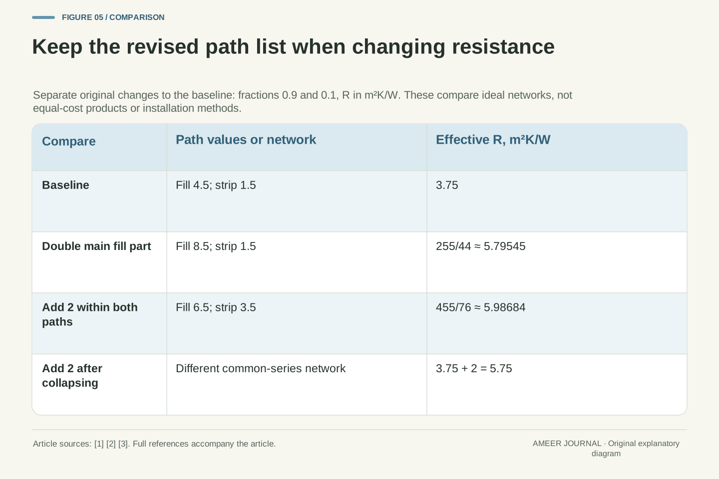
Suppose the main insulating part in the fill region changes from R = 4 to R = 8. Its other-layer contribution remains 0.5, so the new complete fill path is 8.5, not 9. The strip remains at 1.5. We have changed an assigned resistance while holding the model's areas and other values fixed; no particular product, thickness change or purchase is implied.
Apply the same rule again: 0.9 ÷ 8.5 + 0.1 ÷ 1.5 gives a whole-wall U of about 0.172549 W/(m²K). The effective R is about 5.79545 m²K/W. Multiplying U by 10 m² and 20 K gives about 34.5098 W. This is about 35.3 percent below the original 53.333 W, rather than half of it. The calculation has rebuilt the full path and then combined the two regions [1][2].
The strip still carries 13⅓ W. Its share of the now-smaller total rises from 25 percent to about 38.6 percent. A growing percentage does not mean that the strip's absolute heat flow increased. Its own area, resistance and boundary difference did not change. Keep the share and the rate in separate columns when interpreting the result.
Change only the fill material contribution from 4 to 8 m²K/W. The complete path becomes R_f,new=8+0.5=8.5 m²K/W, while R_b=1.5 remains fixed. This distinction matters: doubling one contribution is not doubling its complete series path. Reapply the parallel balance to the revised complete values [1][2].
The new U is 0.9/8.5+0.1/1.5=44/255 W/(m²K), giving R_eff,new=255/44≈5.79545 m²K/W. At the unchanged area and temperature difference, P_new=1760/51≈34.5098 W. Dividing by the baseline 160/3 W gives 11/17; the relative reduction is 6/17≈35.294 percent. The main lesson here is the aggregation procedure: neither the original material R nor its change can stand in for the recalculated complete network.
The strip's absolute rate remains 40/3 W, but its share becomes (40/3)/(1760/51)=17/44≈38.636 percent, compared with 1/4 initially. The share rises because the denominator falls. This example makes no claim of an interaction that increased strip conduction; independence and fixed endpoint temperatures remain explicit assumptions.
Adding resistance to both paths still requires the same aggregation order
Return to the original wall. In a separate change, add R = 2 within each of the two independent paths. Their complete values become 6.5 and 3.5 m²K/W. This is a different hypothetical change from improving only the fill. It does not compare equal costs, equal quantities of material or competing installation methods.
Combining the revised paths gives an effective R of about 5.98684 m²K/W. It is tempting to take the old equivalent 3.75 and simply add 2, obtaining 5.75. That shortcut describes a different arrangement: a single extra resistance attached in series to an already combined wall. Our declared model instead adds resistance inside each path while keeping those paths independent. The two operations do not generally give the same number.
A real layer covering framing as well as a cavity can address both regions, as PNNL explains qualitatively [3]. But a real continuous layer may also let heat move sideways between them. Our two-column arithmetic does not establish that layer's exact performance. The useful lesson is to preserve the stated network when doing the calculation, rather than changing its connections halfway through.
For a separate baseline modification, add r=2 m²K/W to each independent full path. The new values are R_f+r=6.5 and R_b+r=3.5. The equivalent transmittance is 0.9/6.5+0.1/3.5=76/455 W/(m²K), so the effective resistance is 455/76≈5.98684 m²K/W and the total rate is 3040/91≈33.4066 W.
In contrast, R_eff,baseline+r=3.75+2=5.75 m²K/W would yield 800/23≈34.7826 W. The resistance difference is 9/38≈0.236842 m²K/W. Combining a parallel network and then placing a common resistance in series is not the same graph as adding that resistance within every independent branch. A common series element presumes an appropriate common temperature node; that assumption was not introduced into our independent-column model [2].
PNNL supports the qualitative idea that insulation extending across framing can affect its heat-transfer route [3]. The exact behavior of a real sheet also depends on lateral coupling and geometry. These calculations therefore compare two specified ideal networks, not competing construction prescriptions. The original branch definitions must survive any numerical reduction if the resulting equivalent is to answer the same question.
A precise number still belongs to a particular model
Our wall has only two complete paths, fixed properties, common endpoint temperatures and no sideways heat exchange. Those choices make the arithmetic transparent. They also define its reach. If heat spreads sideways, if another connection crosses the wall, or if temperatures change while energy is stored in the materials, the original two independent rates are no longer a complete description.
OpenStax warns that a simple equal-area conduction treatment does not resolve more general three-dimensional heat flow [1]. The same care applies here: a sketch that looks like two regions is not enough to prove that they behave independently. PNNL's framing example explains why another path deserves attention, but it does not supply the areas or resistance values for this invented wall [3].
This does not make the equivalent R useless. It answers a clearly stated question about a particular arrangement. It also helps identify missing information in a real rating: which layers were included, which boundaries were used and how bridges were represented. A calculation with more decimal places cannot fill those gaps. Its precision should not be confused with knowledge of the actual wall.
The reduction to U_eff=Σf_i/R_i assumes independent one-dimensional columns between common fixed temperature boundaries, positive assigned full-path resistances and steady conditions. The expression is exact for that declared network. It does not determine whether the network is an adequate approximation to a physical assembly with multidimensional heat spreading.
OpenStax explicitly limits its simple equal-area series treatment when geometry introduces three-dimensional flow [1]. In our construction, introducing lateral conductance would likewise add connections between intermediate nodes, changing the balance equations. Extra penetrations, time-dependent storage or different boundary conditions would require additional variables rather than a relabeling of the existing equivalent R. PNNL's discussion of framing establishes a qualitative route concern, not a numerical calibration of this model [3].
Keep the level of evidence visible. We have stipulated the network and derived its equivalent; we have not inferred the network from a measured heat rate or validated a particular assembly. Different internal arrangements can share an equivalent resistance at specified conditions. Consequently, an aggregate value alone does not uniquely recover the layer structure or identify which physical detail caused the observed performance.
Ask which quantity was averaged and what each value includes
When reading a wall-resistance calculation, start with the units and the boundaries of each listed value. Is it a material contribution, a complete path or an already combined assembly? Does area remain separate? Then ask how the regions connect. Layers encountered successively within one equal-area path use a different combination rule from side-by-side paths that share endpoint temperatures [1][2].
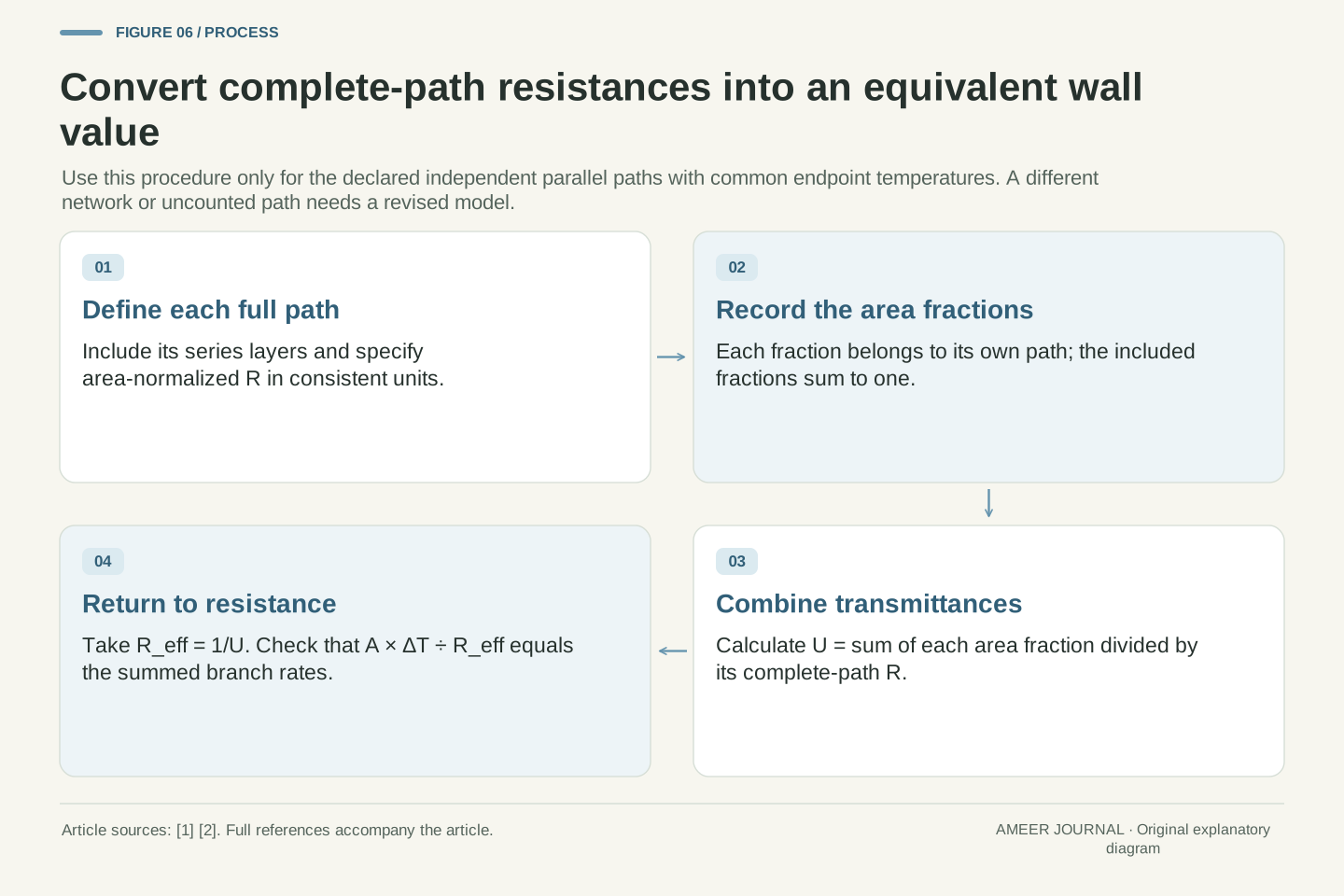
For the independent parallel case, record each complete-path R and its share of the total area. Divide each share by its R, add those results to obtain U, and take the reciprocal if you want the effective R. Check that the fractions cover the intended area and that omitted paths have not disappeared merely because they are small. Recalculate after a change rather than carrying an old equivalent through a different network.
Our original wall has path values 4.5 and 1.5, area shares 90 and 10 percent, and effective R = 3.75 m²K/W. The arithmetic average 4.2 describes a different statistic and predicts too little heat flow for this model. Keeping the path list beside the calculation makes the distinction understandable: the equivalent resistance must reproduce the heat carried by the paths it represents.
An inspectable aggregation record identifies the resistance convention, complete path boundaries, areas or normalized area fractions, common temperature endpoints and permitted connections. Series addition applies within the stated equal-area path; parallel aggregation preserves total conductance between common endpoints [1][2]. These are statements about network structure, not interchangeable operations on a column of numbers.
For independent parallel columns, calculate U_eff=Σf_i/R_i with Σf_i=1, then R_eff=1/U_eff. If using component resistances instead, convert each with its own area before combining reciprocal values. Verify the equal-resistance and vanishing-area limits, and compare the reconstructed total rate with the sum of branch rates. A passing range check alone is insufficient, as both 3.75 and the incorrect 4.2 fall between the original path values.
The numerical result should retain its model identity. Here 3.75 m²K/W is an equivalent for the specified 10 m² two-column wall at the assigned fixed properties; 4.2 is its arithmetic resistance average. A later modification may change a path value, a fraction or a connection. Preserving that distinction lets the next calculation update the physical assumption that actually changed, instead of treating an attractive single rating as a complete description of the assembly.
Sources & further reading
Explore the references behind this guide. External pages may change after our review.
- 1.6 Mechanisms of Heat Transfer - University Physics Volume 2 | OpenStaxOpenStax / Rice University · Accessed 7 Nov 2026
- 16.4 Thermal Resistance CircuitsMassachusetts Institute of Technology, Unified Engineering · Accessed 7 Nov 2026
- Reduced Thermal Bridging | Building America Solution CenterPacific Northwest National Laboratory, Building America Solution Center · Accessed 7 Nov 2026
Article updated 7 Nov 2026.
Found something we should revisit?
Good explanations get better with thoughtful feedback.