What you’ll take away
- Ground sample distance, delivered cell size and sensor response describe different spatial properties.
- Detecting a contrast contribution does not automatically resolve its outline, count or identity.
- A feature’s position relative to a grid can change individual cell values without changing its area.
- Mixed values require a stated model and component information before they can support area estimates.
- Ordinary resampling adds grid entries without collecting new ground observations.
A ten-metre label does not answer every visibility question
A satellite image is labelled “10 m”. You want to know whether it can show a small building, separate two nearby features, or reveal that something bright is present. Those are different requests. The label needs an explanation before it can answer any of them: does it describe the spacing of collected measurements, the grid in the delivered file, or a measure of the sensor's response?
NASA researchers make this distinction in a public presentation abstract. They explain that an image can be placed on an arbitrarily fine grid without changing the sensor's underlying spatial resolution. [1] A large, smooth-looking image therefore does not establish that every displayed square contains a new, independent ground observation. Conversely, the British Antarctic Survey notes that a sufficiently contrasting feature can sometimes be detected even when it is smaller than a pixel. [3]
We will follow one original paper example: a two-metre bright square inside a grid of ten-metre cells. Its signal changes with its position relative to the grid. The exercise uses chosen shapes and values, not a satellite photograph or a detector test. It will show why noticing a contribution, recovering an outline and identifying an object require different evidence.
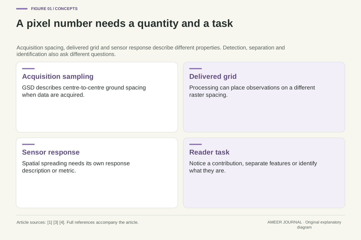
A statement such as “10 m imagery” leaves the relevant spatial quantity underspecified. Acquisition ground sample distance, delivered raster spacing and a sensor-response measure can differ. A user also needs a task definition: detecting a departure from background, resolving separate features and assigning a semantic identity are not equivalent requirements.
The NASA presentation abstract explicitly distinguishes gridded pixel size from sensor spatial resolution, while BAS distinguishes visible-feature scale, raster pixel size and collected GSD. [1][3] These distinctions prevent two opposite errors: treating a finer output grid as new observations, or treating the grid spacing as a universal lower bound on any detectable contrast contribution. Neither follows from the number alone.
The original construction below is a flat-ground, noise-free area-averaging model with ten-metre square cells. It deliberately omits optical blur and other acquisition effects so that one information-loss mechanism can be examined exactly. All shapes, signal values, flags and output arrays are stipulated; no satellite image, classifier or GIS implementation was evaluated. The analysis concerns what that declared representation can distinguish, not a performance estimate for a named instrument.
Read acquisition spacing, delivered spacing and blur separately
Ground sample distance, usually shortened to GSD, describes the distance between sample centres on the ground at acquisition. BAS explains that viewing angle and terrain can affect it. [3] A delivered map also has a grid whose cells have stated dimensions. Processing can place the measurements onto a different grid, so the file's cell spacing needs to be read alongside the acquisition information.
There is another question: how sharply does the sensor respond to a boundary? A sharp ground edge can be represented by a gradual change across image values. In their abstract, the NASA researchers describe examining line and edge responses and reporting the width of a line response at half its maximum height. [1] That is a stated method for characterizing response, not a promise that all useful information stops at a sharp square boundary.
Zooming changes yet another thing: the size of the image on your screen. Esri's documentation distinguishes display scale from the ground dimensions represented by a raster cell. [4] Enlarging a ten-metre cell may make it easier to inspect, but it does not turn the cell into a smaller ground measurement. Keep those three questions visible: where measurements were sampled, how they were spread, and how the result was gridded.
Use acquisition GSD for centre-to-centre spacing on the ground, delivered cell size for the raster's coordinate grid, and an explicitly named response metric for effective spatial spreading. The BAS account notes that acquisition geometry and terrain can vary GSD. [3] A single nominal spacing need not describe every direction and location in an actual acquisition.
The NTRS evidence is the public presentation abstract, not its full results. Its authors describe line-spread-function measurements, or an edge-spread function differentiated to obtain a line response, and use full width at half maximum as their reported spatial-resolution measure. [1] We do not equate that width with GSD or interpret it as a hard-edged footprint. A width at one response level does not define zero response everywhere outside it.
Display magnification leaves the raster's stored grid unchanged, as Esri explains. [4] Resampling changes the representation grid, while new acquisition changes the observations available. Those operations need separate metadata. Our upcoming square-cell model uses uniform weights within each cell and zero weights outside; that is an analytical simplification, not an assertion that real optical sensors have identical rectangular spatial responses.
Noticing, separating and identifying are different tasks
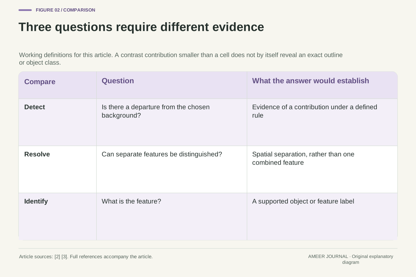
For this article, “detect” means deciding that the values contain evidence of a departure from the chosen background. “Resolve” means distinguishing separate features rather than a single combined feature. “Identify” means determining what a feature is. These working definitions describe the questions we ask; they are not a universal test standard or a fixed rule about pixels per object.
A bright contribution might make one cell look unusual without outlining the thing that caused it. Two small bright patches might also contribute to the same cell. If their combined value matches that of one larger patch, that value alone cannot tell you which scene produced it. The mixed-pixel problem matters because ground objects rarely line up perfectly with the image grid. [2]
This also explains the care needed with the phrase “too small to see”. BAS allows for detecting some smaller features when their contrast dominates the background. [3] That possibility does not establish reliable recognition of every object of that size. Ask which task the evidence supports. A visible difference in a cell, a separated pair of outlines and a confident object label should not silently become the same claim.
Define the inference target before assigning a resolution requirement. Here detection is a decision about a departure from a specified background; resolution is discrimination between spatially separate features; identification assigns a feature type. These operational meanings are chosen for the discussion and do not import a particular military, photographic or machine-vision acceptance criterion.
Their evidence requirements differ even in a deterministic model. A nonzero measurement can indicate a signal contribution, while several underlying scenes map to that same measurement. In that case, the mapping does not support a unique object count or shape. BAS's mixed-pixel explanation motivates this concern: real boundaries generally do not coincide with raster boundaries. [2]
The BAS spatial-resolution guide also notes that subpixel features can sometimes be detected through sufficiently dominant contrast. [3] This is a qualified possibility, not a sensitivity guarantee. In a real task, the background, noise, response, decision rule and available contextual evidence must be specified. The examples below demonstrate non-uniqueness directly, without assuming that a selected detection threshold is a calibrated statistical procedure.
Build a simple cell value from area and contrast
Imagine a flat twenty-metre square divided into four equal cells. Each cell is ten metres wide and ten metres tall, so its area is one hundred square metres. For this exercise, the background has signal value zero and a bright square has value one hundred. These are arbitrary signal units, not temperatures, percentages of reflected sunlight or measured satellite values.
Our pretend sensor reports the average value over each cell. Put a two-metre by two-metre bright square completely inside the lower-left cell. The patch occupies four square metres out of one hundred. Four percent of that cell contributes value one hundred and the rest contributes zero, giving a cell average of four. The other three cells remain zero.
That average is not a drawing of the patch. It says how the supplied values combine under our rule. Many patch positions within the cell produce the same answer. Real pixels can contain contributions from different surfaces, as BAS explains, [2] but real weighting can be more complicated than our square average. We have chosen a simple rule so that the hidden information is easy to see.
Let the extent be [0,20] × [0,20] metres, divided at x=10 and y=10 into four cells of area A=100 m². Set the background signal b=0 and the patch signal o=100 in arbitrary common units. Define each observation as the uniform area mean over its cell, with no blur, noise or atmospheric term.
If a patch overlaps a cell by area a, that cell's value is y=(a/A)o+(1−a/A)b. For a two-metre square wholly inside one cell, a=4 m² and y=(4/100)×100=4. In the order lower-left, lower-right, upper-left, upper-right, the observed vector is (4,0,0,0). Area fractions are dimensionless; the mean retains the chosen signal unit.
This is an explicit forward model. It combines a scene into four observations; it does not promise a unique inverse. The BAS discussion supports the general concern about mixed contributions, [2] while this exact formula and geometry are our construction. Different locations, outlines or component values can produce the same means, even before any real sensor blur or measurement uncertainty is introduced.
Move the same patch across a boundary and its contribution splits
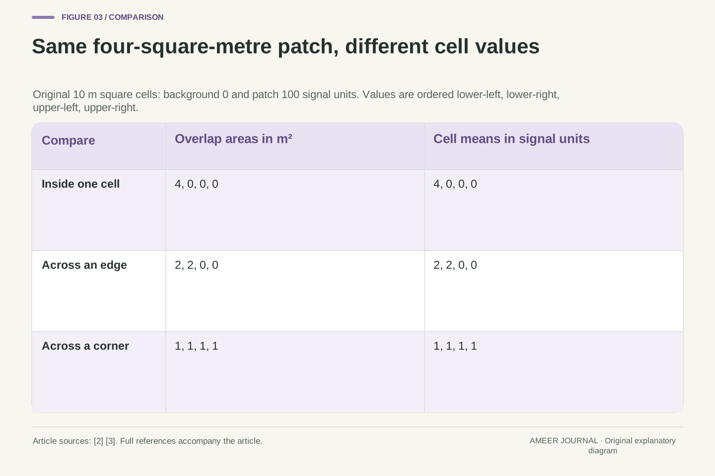
Compare three separate placements of the same bright square. First it sits wholly inside one cell, producing values 4, 0, 0 and 0. Next it straddles the vertical boundary halfway across its width. Each of two cells receives two square metres of the patch, producing 2, 2, 0 and 0. Finally it is centred on the four-cell crossing. Each cell receives one square metre, giving 1, 1, 1 and 1.
The square has not changed size or brightness. What changed was the distribution of its contribution across the grid. The sum of the four values is four in every case, but the largest single-cell value falls from four to two to one. A rule that looks only at individual cell values can therefore respond differently to the same kind of feature in different positions.
The accounting also has a useful check. Multiply each cell value by its one-hundred-square-metre area and add the results. Each scene gives four hundred signal-unit square metres, matching four square metres of patch at value one hundred. This is conservation within our averaging construction. It is not an observation that a real satellite's measured response must be independent of position.
Use patch rectangles x∈[4,6], y∈[4,6] for the inside case; x∈[9,11], y∈[4,6] for the edge case; and x∈[9,11], y∈[9,11] for the corner case. Coordinates are metres. The overlap areas with the four cells are respectively (4,0,0,0), (2,2,0,0) and (1,1,1,1) m².
With o=100, b=0 and A=100 m², the numerical mean vectors are the same tuples in signal units. Their sums are all four, whereas their maxima are four, two and one. These are three stipulated scene placements, not sampled motion or an experimental shift test. Feature/grid alignment is the only changed variable in this construction.
The area-weighted sum is ΣA y=400 signal-unit m² for every placement, equal to patch area multiplied by its signal. An unweighted sum of means would not serve as an area integral if cell areas differed. Here the common area makes the check immediate. The example isolates spatial mixing associated with boundaries [2]; it does not assert the same exact invariance under a nonuniform real sensor response.
A missed flag is not an absent object, and one flag is not one object
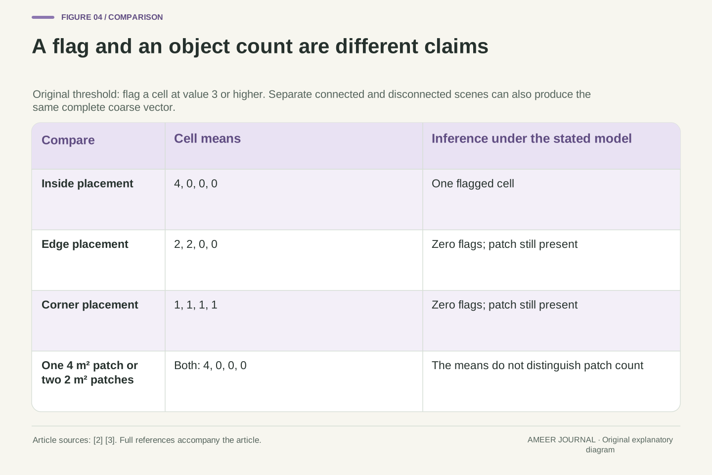
Now invent a simple flag: mark a cell if its value is at least three. The inside placement produces one flag. The edge and corner placements produce none. Every scene still contains the bright square. Our flag counts describe this chosen rule, not a tested detector's accuracy or the probability of finding an object.
There is a second ambiguity even when a cell is flagged. Compare the original two-metre square with two separated rectangles, each one metre wide and two metres tall, both wholly inside that same cell. The single square covers four square metres. The pair also covers four. At the same signal value, both scenes give the identical four-cell values: 4, 0, 0 and 0.
One bright cell therefore cannot settle whether the scene contains one connected patch or two disconnected patches under this model. Nor does it recover their positions inside the cell. The information has been combined before the viewer sees the grid. Adding a stronger object label to the same value does not supply the missing distinction; that inference would need additional measurements, assumptions or contextual evidence.
Define the original deterministic flag D(y)=1 when y≥3 and D(y)=0 otherwise. Applied cell by cell, the three placements yield flag counts 1,0,0. The rule is intentionally arbitrary: no background distribution, noise model, false-positive rate or empirical threshold selection is supplied. It cannot be interpreted as a calibrated detection probability.
For a stronger non-uniqueness example, compare the single patch [4,6] × [4,6] with two disjoint patches [2,3] × [4,6] and [7,8] × [4,6]. The latter each have area 2 m² and remain inside the lower-left cell. With the same o and b, both scenes produce exactly (4,0,0,0).
The forward map is therefore many-to-one for these candidate scenes. No deterministic inference using only that four-value vector can be correct about connectivity or patch count for both scenes without introducing other information. This conclusion is exact within the stated model. It does not prohibit real methods from using additional bands, observations, spatial context or prior assumptions; it requires those additions to be named rather than attributed to the cell spacing alone.
A brighter cell does not uniquely reveal the covered area
Suppose all you know is that one cell has value four. Our first example explained it using a four-percent area fraction at signal one hundred. A different scene also works: eight percent of the cell at signal fifty, with the same zero background. Eight percent of fifty is four. The contributing area has doubled while the observed mean stays unchanged.
To recover an area fraction from a mixed value, you need more than the mixed value. You must know the signals assigned to the two components and assume that the averaging rule is valid. If those conditions hold, you can work backwards through the weighted average. If they do not, a confident-looking percentage can hide an unsupported choice of component brightness.
Even a correctly recovered area fraction would not give the patch outline or the number of patches. Four percent could be arranged in several ways inside the cell. This is why mixed pixels deserve attention in image analysis. [2] The quantities a model can estimate depend on its assumptions and evidence; a display's neat grid does not make every underlying ground property separately observable.
Write the two-component model as y=(1−f)b+fo, where f is the patch's area fraction. If o and b are known and o≠b, algebra gives f=(y−b)/(o−b). The inverse requires both the component values and the validity of the linear two-component model; it does not follow from pixel spacing alone.
For y=4 and b=0, choosing o=100 gives f=1/25=0.04, or 4 m² in the cell. Choosing o=50 gives f=2/25=0.08, or 8 m². An explicit eight-square-metre rectangle [3,7] × [4,6] at signal fifty produces the same four-cell observations as the original square at signal one hundred.
These are constructive alternatives, not a real spectral-unmixing result. A single known fraction would still leave shape, connectivity and location within the cell unspecified. BAS's mixed-pixel warning [2] motivates checking such assumptions, but it does not validate our arbitrary component values for an actual scene. Interpreting a numerical estimate requires retaining the forward model and the information that made its unknowns identifiable.
A finer output grid can repeat information instead of adding it
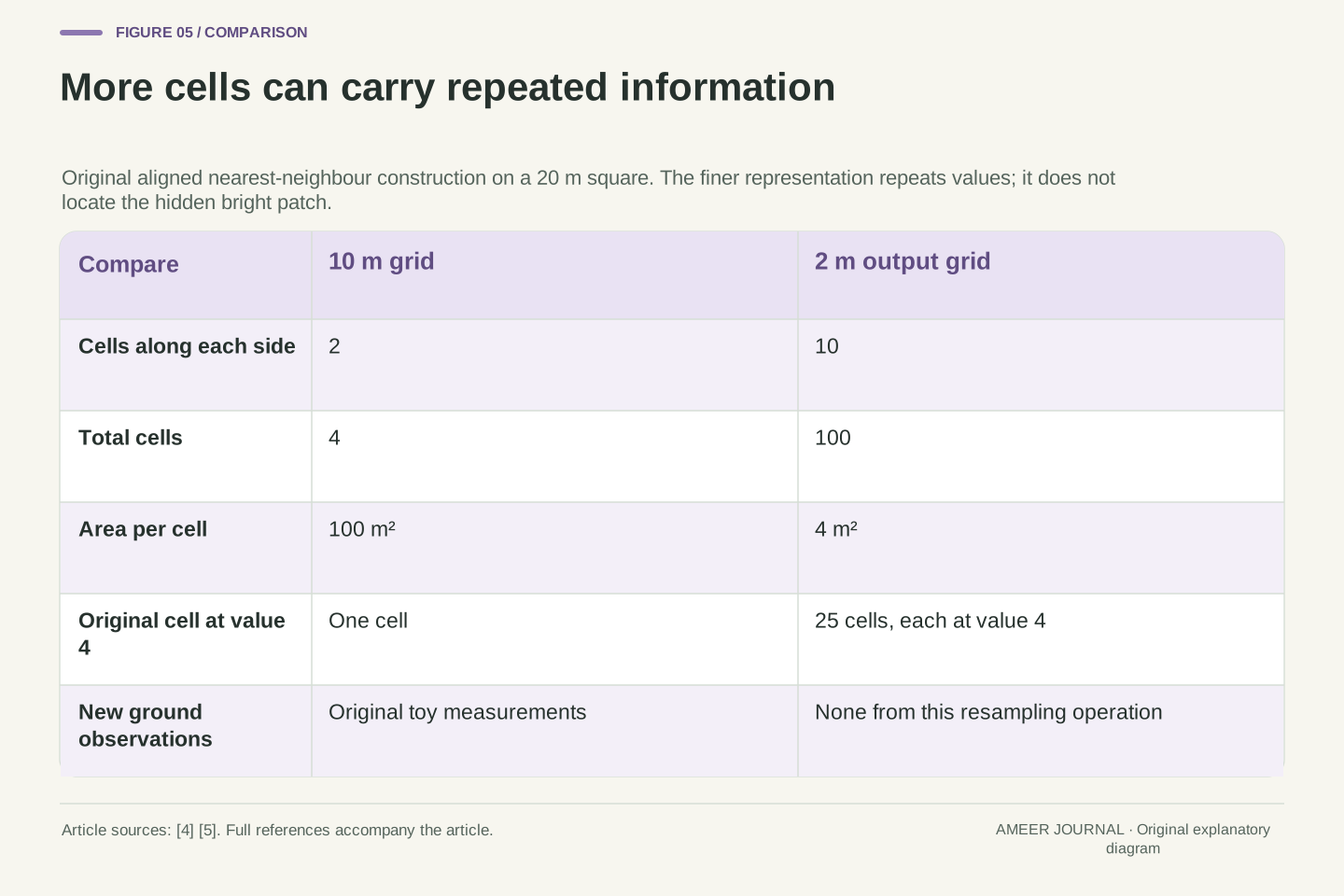
Return to the twenty-metre square containing four ten-metre cells. Re-express the same extent using two-metre cells. There are now ten cells along each side, or one hundred cells altogether. That is twenty-five times as many entries. It does not mean the satellite collected twenty-five times as many ground observations. Esri explicitly warns that resampling to smaller pixels does not produce greater detail. [4]
For a clearly defined example, align both grids and use nearest-neighbour assignment. Each original cell becomes a five-by-five block of twenty-five smaller cells carrying its old value. The original cell with value four becomes twenty-five cells with value four. Nothing in this operation reveals where its hidden bright patch was located. Nearest-neighbour assignment uses source values; it does not measure the ground again. [5]
Our original two-metre square happens to fit one of the new small cells exactly. The true toy scene on that fine grid would have one cell at one hundred and the others at zero. Repetition instead paints twenty-five cells at four. Both give the same total under the coarse average, but their fine arrangements differ. More grid entries have not selected the correct hidden arrangement.
For fixed extent 20 m × 20 m, a square grid of spacing 10 m has 2×2=4 cells; spacing 2 m has 10×10=100 cells. The count ratio is (10/2)²=25. This is an exact nested-grid construction with aligned boundaries, not a simulation of all ArcGIS extent, projection, rounding or nodata behavior. [5]
Nearest-neighbour assignment repeats each source value into a 5×5 output block in this geometry. [5] For the inside-patch scene, the output has twenty-five entries of four and seventy-five of zero. Each fine cell covers 4 m², so its area-weighted sum remains 25×4×4=400 signal-unit m². That preservation follows from the chosen replication and alignment, not a claim about arbitrary resampling.
The underlying two-metre square at [4,6] × [4,6] would instead yield one fine cell of one hundred and ninety-nine zeros under the fine area-mean rule. Replication cannot choose that hidden arrangement from the coarse vector. Esri's smaller-pixel warning [4] fits this distinction: ordinary regridding changes the representation, while it supplies no new observation that distinguishes scenes already identical on the input grid.
Smoothing and category labels need different treatment
A smoother result can be useful without being a new measurement. Esri describes bilinear interpolation as a weighted combination of four nearby input-cell centres. [5] Unlike simply copying one source value, it can create intermediate values. That changes how a transition looks and how the output numbers should be interpreted.
The type of number matters too. A continuous signal value can sensibly enter a weighted average under an appropriate model. A category code is a label. If numbers stand for land-cover classes, averaging those codes does not automatically describe a mixture of the classes. Esri therefore advises against bilinear and cubic methods for categorical data, where altered values can be inappropriate. [5]
When comparing a small-cell image with its source, record the resampling method and what the values mean. Did the process copy values, combine neighbours or use additional information? A pleasant edge is not enough to answer. Ordinary interpolation operates on the supplied raster; any claim to infer previously unresolved structure needs its own method, assumptions and validation. That claim cannot be established by the destination cell size.
The pinned ArcGIS Pro 3.4 documentation distinguishes nearest-neighbour assignment from bilinear interpolation, which combines the four nearest input-cell centres using distance-related weights. [5] These definitions describe how output values are obtained. They do not make the destination grid an independent acquisition or turn smoothing into a sensor-resolution measurement.
Categorical values require separate semantics. A numeric class code is not necessarily an interval-scale measurement, so an arithmetic combination can yield a code whose meaning is unrelated to the source classes. The documentation warns against bilinear and cubic resampling of categorical data for this reason. [5] We do not execute either method or infer a universal best choice for every dataset.
For a deterministic resampler with the same settings, identical input arrays give identical output arrays. The two hidden scenes that produced our common coarse vector remain indistinguishable through such resampling alone. A reconstruction method using extra observations or explicit priors changes the evidence or assumptions; it needs to be assessed on those terms. This distinction preserves a useful role for interpolation without crediting it with measurements it never collected.
A documented thermal-band example has two different spacings
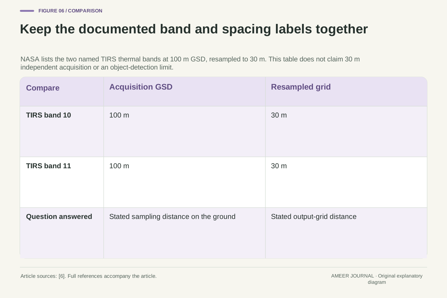
The distinction appears in real mission documentation. NASA's TIRS table lists thermal-infrared bands 10 and 11 with a one-hundred-metre ground sample distance, resampled to thirty metres. [6] The thirty-metre grid is therefore not, by that description alone, evidence that those thermal measurements were independently collected every thirty metres.
Read the band names as part of the statement. This example concerns the two specified TIRS thermal bands; it does not describe every band from every Landsat instrument. It also does not tell us a particular line-response width or prove that a thirty-metre ground object can be identified. Those questions require the relevant response and task evidence.
Do not transfer the exact twenty-five-copy result from our toy grid to this product. Ten metres divided by two was an integer ratio with deliberately aligned cells. One hundred divided by thirty is a different ratio, and no actual TIRS output file or resampling implementation was examined here. The documented example contributes a narrower, useful fact: acquisition sampling and a delivered grid can carry different spatial numbers.
NASA's TIRS spectral-band table gives bands 10 and 11 a GSD of 100 m, resampled to 30 m, and defines GSD as ground distance between pixel centres. [6] This provides a concrete distinction between acquisition sampling and output-grid spacing. The named band scope is essential; it is not a statement about every Landsat channel or product.
Neither number alone supplies an effective line-spread-function FWHM, a calibrated detection threshold or a semantic-recognition rate. Those quantities require other definitions and evidence. Likewise, a resampled thermal cell is not established as an independent 30 m acquisition merely because that is its grid dimension.
Our integer replication factor belongs only to the original 10-to-2 m nested grids. The 100-to-30 m example has a different ratio and unspecified processing details for this discussion. No file-level geometry, alignment or actual data array was inspected. Keeping the published sampling statement separate from our arithmetic prevents a legitimate mission example from becoming an invented reconstruction of its implementation.
Write down the task before judging the pixel number
When the next image offers a resolution number, begin with your question. Are you looking for a possible change, trying to separate two features, or assigning an identity? Then find the acquisition sampling information, the delivered grid dimensions, any available response description and the processing method. The sources distinguish these quantities because each answers a different part of the problem. [1][3][4][5]
Our bright-square exercise gives a practical reason for that care. The same patch produced one, two or four nonzero cells depending on placement. A fixed flag missed two placements, and a single connected patch could share its entire coarse image with two disconnected ones. Finer replication increased the number of entries without choosing between those scenes.
A useful description therefore says what the image values support and what additional inference is being made. Keep the band, time, geometry and processing context attached when they matter to the real task. A pixel-spacing label is valuable information. It becomes misleading when it is asked to stand in for an object outline, a count, an identification or a demonstrated detection result that has not been established.
A defensible interpretation record links a defined task to acquisition GSD, delivered grid, coordinate geometry, relevant sensor-response information and transformation history. Product and band identifiers preserve the scope of those quantities. NASA's response discussion, BAS's GSD account and Esri's display/resampling guidance explain why none of these fields substitutes for the others. [1][3][4][5]
The original calculations establish specific limits: equal-area placements alter per-cell maxima; a fixed threshold is placement-dependent; different patch counts and contrasts can share the same observations; and an aligned finer grid can expand cardinality without resolving that ambiguity. These conclusions follow from the declared averaging model, not from an empirical assessment of satellite capabilities.
For a real application, evaluate the proposed inference using the relevant observations, uncertainty and validation rather than a universal pixels-per-object slogan. Additional measurements and justified assumptions may support more than a single raster does, but they must remain visible in the explanation. The final question is what distinguishes the competing ground scenes in the evidence you actually have.
Sources & further reading
Explore the references behind this guide. External pages may change after our review.
- Determining True Sensor Spatial Resolution of Very High Resolution Optical Imagery - NASA Technical Reports Server (NTRS)Alana Semple, Bin Tan and Guoqing Lin / NASA Technical Reports Server · Accessed 7 Nov 2026
- Mixed pixelsBritish Antarctic Survey / Geospatial technical guides · Accessed 7 Nov 2026
- 3. Spatial resolutionBritish Antarctic Survey / Geospatial technical guides · Accessed 7 Nov 2026
- Pixel size of image and raster data—ArcGIS Pro | DocumentationEsri / ArcGIS Pro documentation · Accessed 7 Nov 2026
- Resample (Data Management)—ArcGIS Pro | DocumentationEsri / ArcGIS Pro documentation · Accessed 7 Nov 2026
- Thermal Infrared Sensor (TIRS) - NASA ScienceNASA / Landsat mission · Accessed 7 Nov 2026
Article updated 7 Nov 2026.
Found something we should revisit?
Good explanations get better with thoughtful feedback.