What you’ll take away
- Polarization describes electric-field behavior across propagation; it is distinct from frequency and travel direction.
- Under the controlled linear model, voltage follows cos θ and received power follows cos² θ.
- A reversed signed voltage can have unchanged power, while an ideal null belongs to one receive channel.
- Circular and unpolarized inputs can produce the same flat mean-power trace in a rotating linear analyzer.
- A mixture calculation needs its stated components and calibration; polarization coupling alone does not predict a complete wireless link.
The radio wave can stay the same while the receiver responds differently
Imagine an ideal receiving antenna connected to a power meter. At one orientation, the meter shows a strong response. Turn the antenna through a right angle and its response falls to zero in our mathematical example. Nothing about the incoming wave's frequency has changed. The antenna is responding to a different part of the same electric field. This dependence on direction is called polarization coupling. The National Radio Astronomy Observatory explains it through the response of a linearly polarized receiving antenna. [1]
The useful question is not simply whether a radio wave is present. It is how that particular receiver responds to the wave that reaches it. A receiver can miss a component that another receiver would detect. An ideal zero reading therefore does not mean that the space around the antenna contains no radio energy. Nor does a larger reading automatically describe a faster internet connection.
We will use original calculations with an imaginary, carefully controlled receiver. There is no physical antenna adjustment or radio transmission to perform. First we will separate the wave's travel direction from its electric-field direction. Then we will calculate how a tilted receiver changes voltage and power, and finally ask what a rotation experiment could still leave unknown. That last question matters: different polarization states can produce the same power readings.
Consider an ideal linear receive channel exposed to a monochromatic, fully linearly polarized plane wave. The incident frequency, propagation direction and field amplitude are fixed. Comparing stationary receive-axis orientations changes the channel's response even though the incident wave is unchanged. NRAO gives the voltage dependence as cos θ and the power dependence as cos² θ, where θ measures the relative orientation of the feed and incident electric field. [1]
This is a question about polarization selectivity, not the existence of radiation. A null in one ideal receiver port does not imply zero incident electromagnetic energy. The same distinction prevents a polarization factor from being used as a direct percentage of network throughput, which would require a separate communication-system model.
The original examples below isolate field projection, same-load power detection and the interpretation of angular response. They are not measured antenna data or a software simulation. We will define the geometry before using the cosine law, preserve the sign of voltage before squaring, and compare linear, circular and unpolarized inputs. In particular, a constant reading from a rotating linear analyzer does not uniquely identify an unpolarized input. That ambiguity limits what can be concluded from a power trace alone.
The electric field points across the direction of travel
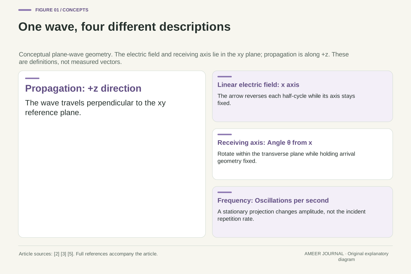
For the simple wave in this article, draw its travel direction straight toward you. The electric field moves side to side in a plane across that direction. In a linearly polarized wave, it oscillates along one fixed line: it points one way, passes through zero, and points the opposite way. Its axis stays the same even though its arrow reverses. NRAO's wave primer distinguishes this electric-field behavior from the direction in which the wave propagates. [3]
Now put two perpendicular reference lines on that transverse plane and call them x and y. Let the incoming electric field lie along x. A receiving axis can also lie along x, along y, or somewhere between them. The angle we need is between the incoming field's axis and the receiving axis in this shared plane. It is not the angle between the receiver and the wave's travel direction.
Frequency answers a different question: how rapidly the oscillation repeats. Polarization describes the electric field's directional behavior. [2] A smaller sideways projection can have exactly the same repetition rate. Words such as horizontal and vertical only help when the reference frame is known; rotating a drawing on a screen does not change the physical relationship between its two axes.
Use a right-handed coordinate system with propagation along +z. The x and y directions span the transverse plane. For a free-space plane wave, both electric and magnetic fields are perpendicular to propagation; the electric field therefore needs only two transverse components. [2][3][5] These assumptions are specific to the plane-wave description, not a universal statement about every field near an antenna.
Let E(z,t)=E0 x̂ cos(kz−ωt), with E0 a positive field amplitude, k the wavenumber and ω the angular frequency. A real unit receive axis in the same basis is u(θ)=x̂ cos θ+ŷ sin θ. Here θ is an in-plane angle measured from x toward y. Every u remains perpendicular to z, so the incoming direction stays broadside to the ideal linear element.
A linear polarization axis is unchanged by the field's half-cycle sign reversal. Its frequency is determined by ω, whereas its polarization is determined by the relative transverse components and their phase behavior. [2][5] Defining both vectors in the same basis is essential: a dot product between coordinates expressed in unrelated local frames has no physical meaning until the frames are related. Horizontal and vertical are labels within that geometry, not universal directions detached from it.
Hold the other reasons for a power change fixed
A real antenna can change its response for several reasons when it moves. It may face the incoming direction differently, encounter a different surrounding field, or behave differently near other objects. Our example deliberately controls those possibilities. The incoming wave stays fixed. The receiving axis rotates only within the plane across the wave's travel direction, and we compare it after it has stopped at each angle.
We also keep the receiver's sensitivity, electrical connection and power measurement unchanged. Its ideal response is purely linear: it selects the electric-field component along its axis. MathWorks describes polarization mismatch through this projection and emphasizes that the field and receiver directions must be expressed consistently. [5] These conditions allow the angle to be the one changing ingredient in the calculation.
Call the aligned received power P0. This is what the same ideal system receives when its axis matches the incoming linear polarization. It is not the transmitter's total output or all the energy passing through the surrounding space. For our invented example, P0 is 16 microwatts, written 16 µW. A microwatt is one millionth of a watt. Every later percentage will refer to that explicitly chosen aligned reading.
The model holds incident flux, arrival direction, receiver sensitivity and electrical loading fixed while varying only the transverse receive-axis orientation. Rotation about the propagation axis preserves broadside geometry for the ideal linear element. Comparisons are between stationary states; no moving-receiver modulation or continuous-rotation sidebands are being modeled.
The channel is an ideal linear polarization selector with unchanged effective response and no cross-polar leakage. Its conversion from projected field to terminal voltage has the same proportionality constant at every orientation. The load and power calibration also remain unchanged. These conditions isolate the normalized projection factor described in the official polarization documentation. [1][5] They would need independent justification before applying the same calculation to a physical assembly.
Define P0 as the time-averaged received power of this system in its aligned state. Normalizing by P0 removes the fixed response scale, leaving a dimensionless polarization factor. It does not assert that the antenna collects all transmitted power or all flux crossing an arbitrary surface. The illustrative P0=16 µW is stipulated, not measured. The polarization calculation then determines relative received powers, while an absolute link budget would still need propagation, aperture, loss and calibration information.
Half the voltage response means one quarter of the power
The receiver first selects a component of the electric field. For our linear wave, the voltage response is multiplied by cos θ, pronounced “cosine theta”. This is the geometric projection onto the receiving axis. When θ is zero, the axes match and the factor is one. At 60 degrees, the factor is one half. NRAO gives this voltage relationship before stating the corresponding power relationship. [1]
Power is not multiplied by that same fraction. With the electrical load unchanged, average power follows the square of the voltage amplitude. Half the voltage response therefore gives one quarter of the power. The complete rule is P=P0 cos² θ: take the cosine, square it, and multiply by the aligned power. The square is what the small raised 2 means.
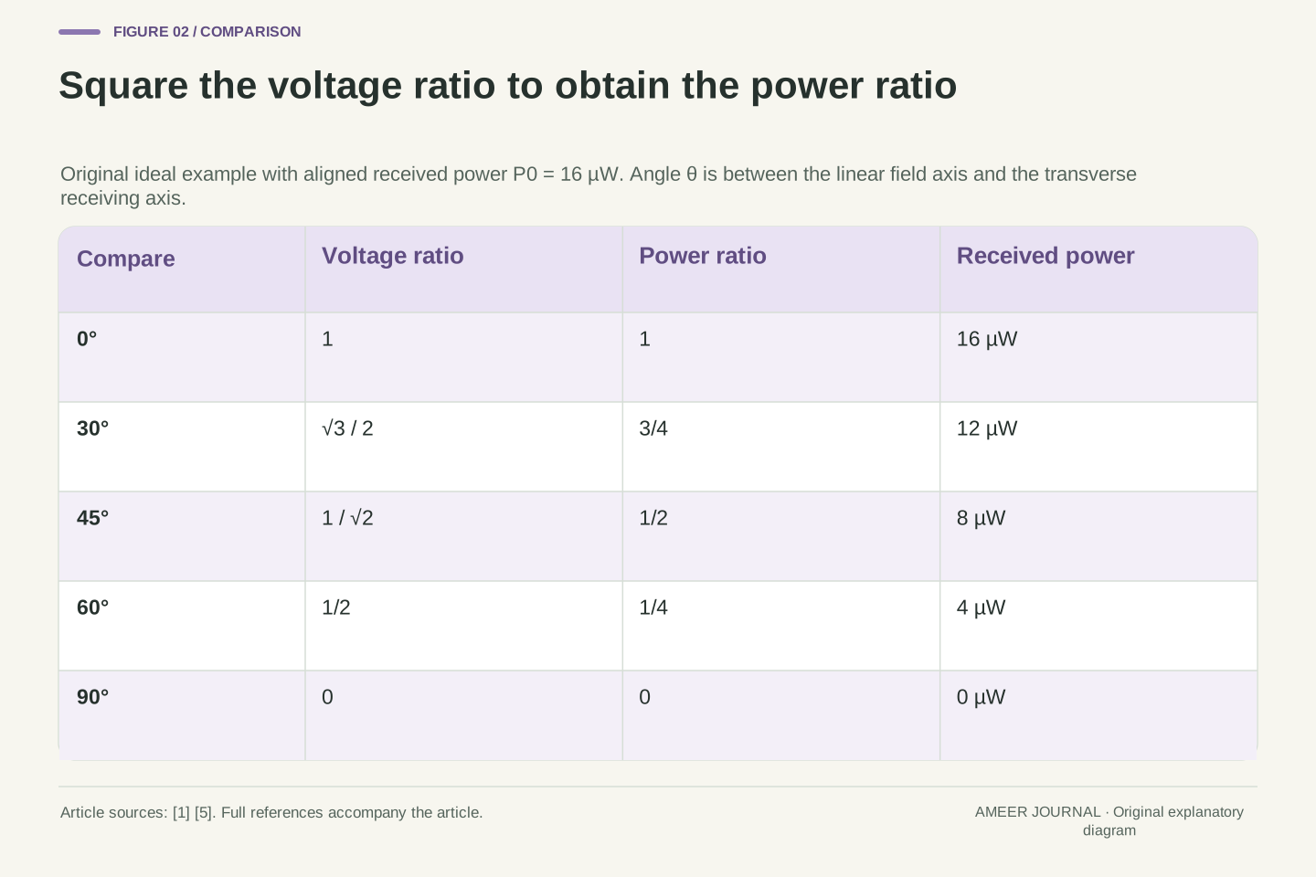
Using our 16 µW reference, angles of 0, 30, 45, 60 and 90 degrees give powers of 16, 12, 8, 4 and 0 µW. At 45 degrees the voltage fraction is about 0.707, whose square is one half. It is not a voltage fraction of one half. None of these stationary projections changes the original oscillation's frequency. The voltage becomes smaller, but it still repeats at the same rate whenever its amplitude is nonzero.
The real-axis projection is u·E=E0 cos θ cos(kz−ωt). With a fixed conversion constant, the corresponding signed voltage-amplitude ratio is Vθ/V0=cos θ. The frequency factor remains unchanged because cos θ is constant for each stationary orientation. NRAO's feed-response relation supplies this cosine dependence. [1]
For a fixed resistive load R, a sinusoidal voltage with peak amplitude Vθ gives mean power Vθ²/(2R). Therefore Pθ/P0=(Vθ/V0)²=cos² θ. The same ratio follows if RMS voltages are used consistently; the peak-to-RMS factor cancels. Using voltage and power ratios interchangeably would omit the square and overestimate the retained power away from alignment.
Our exact power factors at 0°, 30°, 45°, 60° and 90° are 1, 3/4, 1/2, 1/4 and 0. Multiplying by 16 µW produces 16, 12, 8, 4 and 0 µW. At 45°, the amplitude factor is 1/√2; at 60°, it is 1/2. Both checks expose the same distinction between field amplitude and power. These values are exact within the stipulated model, apart from decimal displays of irrational amplitude ratios. The zero case has no nonzero output sinusoid whose frequency could be measured at that port.
A reversed voltage can have the same detected power
Extend the angle comparison to 180 degrees. The receiving axis now points opposite to the incoming field's chosen positive direction. Its signed projection is minus one instead of plus one. With our fixed electrical polarity reference, that means the voltage waveform is reversed: a positive part becomes negative, and a negative part becomes positive. Squaring either waveform gives the same power. [1][3]
An ordinary power value cannot tell these two signs apart. Both the 0-degree and 180-degree cases give 16 µW in our example. Linear polarization describes an axis, so turning that axis through half a full rotation returns the same polarization alignment. The sign still matters when comparing voltage waveforms using a defined reference; it has simply disappeared from this power measurement.
At 90 degrees, the selected component is zero. This does not erase the incoming field. Another ideal receiver aligned with that field would respond to it. The important phrase is “zero in this channel under these assumptions”. Real equipment can have imperfect polarization rejection or receive waves from several paths, so the exact mathematical zero is not a promised meter reading outside the model.
For a directed receive-axis and terminal-polarity convention, cos(θ+π)=−cos θ. The signed voltage amplitude changes sign, equivalent to a π phase reversal for a nonzero sinusoid, but cos²(θ+π)=cos² θ. Thus the power response is periodic in 180°, even though the signed projection changes. [1][3] No claim about an unspecified device's wiring or phase-sensitive output is needed.
This separates a polarization axis from an oriented vector used to represent terminal voltage. The linear state has the same axis after a half turn. Reversing the chosen voltage reference cannot create negative received power; same-load power is quadratic. At θ=0 and θ=π, the illustrative voltage ratios are +1 and −1, while both power ratios equal one.
At θ=π/2, the ideal channel is orthogonal to the incident electric field and its selected component vanishes. This is a response null, not a statement that the incident field or its energy flux vanishes. The conclusion also relies on perfect linear selectivity and the single specified incident wave. Cross-polar leakage, altered arrival geometry or additional fields fall outside the controlled calculation; they must not be silently folded into a claim of an exact real-world null.
A power ratio and a positive loss use opposite signs
Radio descriptions often express a power change in decibels, written dB. A decibel value compares two powers using a logarithm. For this article, the comparison is the received power at an angle divided by the aligned received power. It is a ratio, so the common unit cancels. The calculation does not introduce a new physical loss mechanism; it expresses the same polarization factor in another form. [1][5]
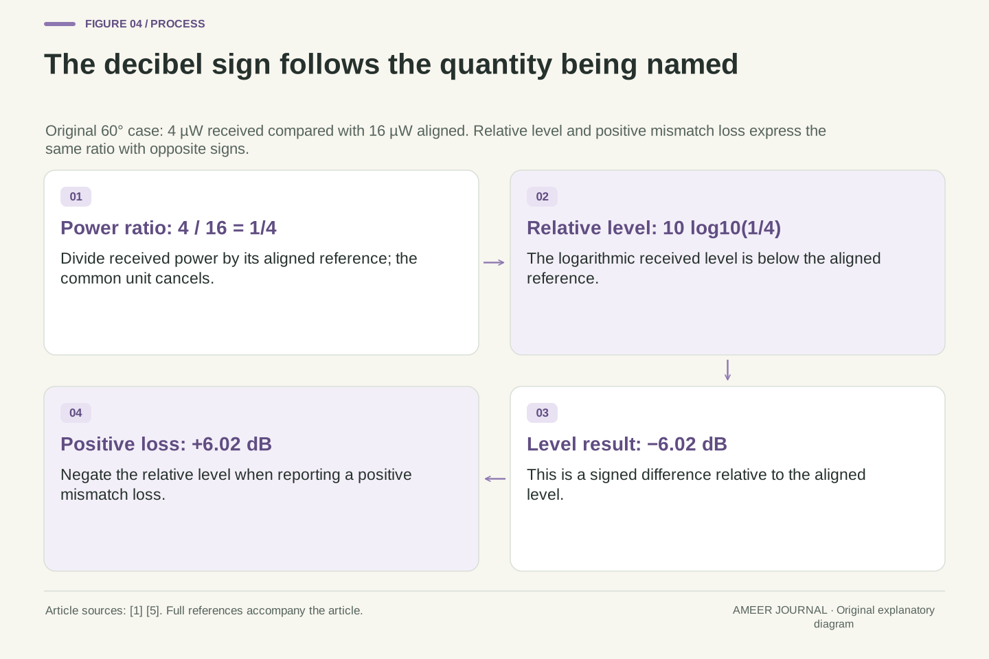
At 60 degrees, our reading is 4 µW instead of 16 µW. The ratio is 4 divided by 16, or one quarter. Ten times the base-ten logarithm of one quarter is about −6.02 dB. This says that the received level is 6.02 dB below the aligned reference. If we instead report a positive “mismatch loss”, its value is +6.02 dB. The sign depends on which of those two quantities the label names.
At 45 degrees, half the aligned power corresponds to about −3.01 dB relative level or +3.01 dB loss. At 30 degrees, three quarters corresponds to about +1.25 dB loss. The ideal zero at 90 degrees has no finite logarithm. Calling its loss infinite describes a mathematical limit, not a finite measured number that a real instrument has established.
For a nonzero power factor ρ=Pθ/P0, define the relative level GdB=10 log10 ρ. A positive mismatch-loss convention instead uses LdB=−10 log10 ρ. These are equal in magnitude and opposite in sign. Because the load is unchanged and ρ=(Vθ/V0)², the equivalent expression is GdB=20 log10|Vθ/V0|. The absolute value is necessary when the signed voltage ratio is negative.
At θ=60°, ρ=1/4 gives GdB≈−6.020600 dB and LdB≈6.020600 dB. At 45°, ρ=1/2 gives a positive loss of about 3.010300 dB; at 30°, ρ=3/4 gives about 1.249387 dB. These original logarithm calculations re-express the cosine-squared power factors supported by the antenna references. [1][5] They are not independently measured attenuation values.
At the exact orthogonal null, ρ=0 and log10 ρ is not a finite real number. The relative level tends to negative infinity as ρ approaches zero from above, while positive loss tends to positive infinity. A real meter's displayed floor, noise or leakage would require another model. Writing a finite instrument reading beside this ideal infinity would confuse an observation limit with the exact response factor being calculated.
A second channel accounts for the perpendicular component
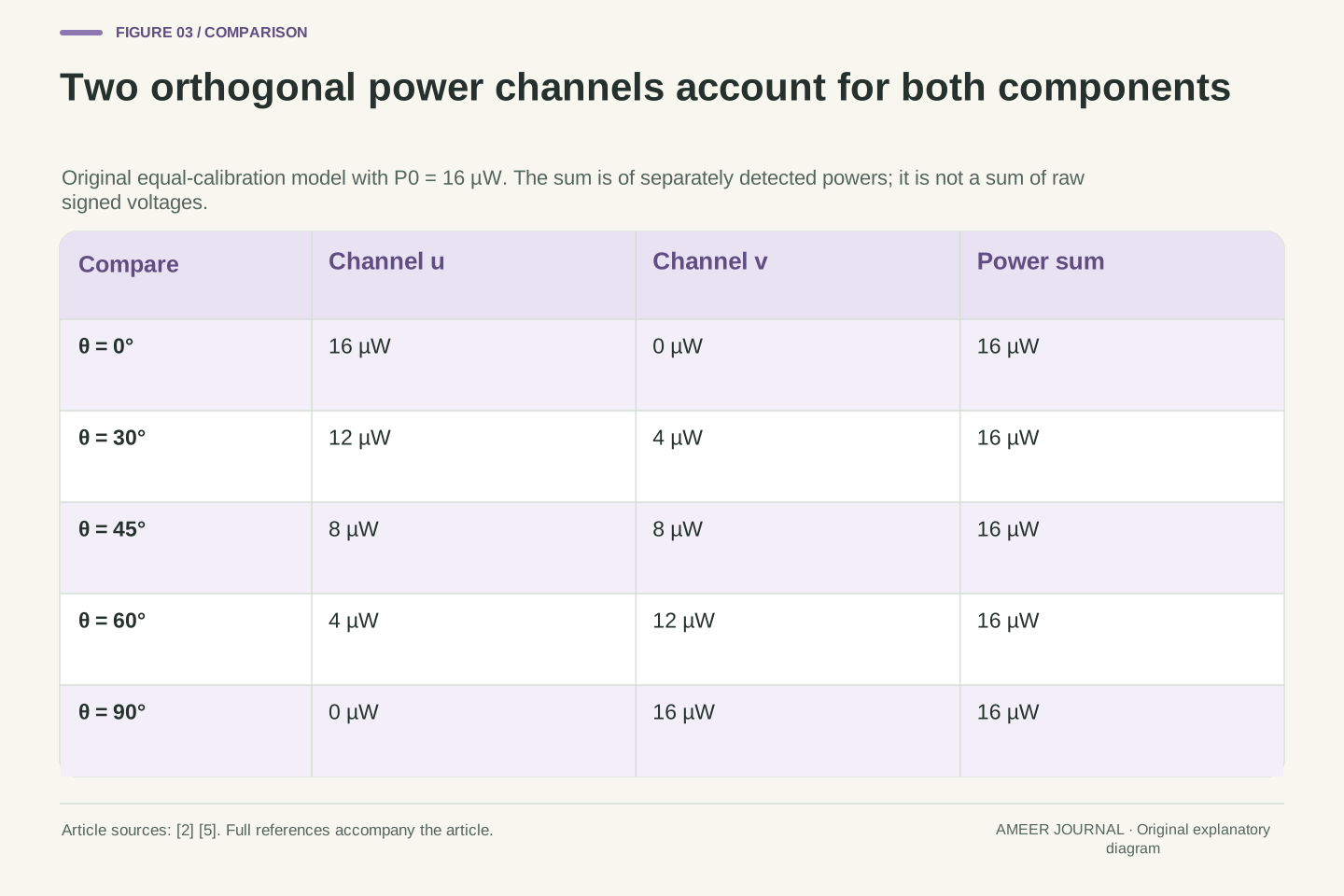
Suppose the imaginary receiver now has two ideal, equally sensitive channels. Their receiving axes remain at right angles to one another. If the first axis is tilted 30 degrees from the incoming linear field, it receives 12 of our 16 µW. The other channel receives the remaining 4 µW. At 45 degrees, each receives 8 µW. When one is perpendicular to the field and receives zero, the other is aligned and receives 16 µW.
The reason is a geometric identity: the squared cosine and squared sine of the same angle add to one. The two channels divide the response into perpendicular components under the shared calibration. NRAO describes the role of orthogonal polarization channels in accounting for both components of radiation. [2] The calculation does not create extra power by drawing a second receiver.
It is important to add the channel powers, not just their signed voltages. Voltage signals can have different signs or timing relationships, and combining them electrically is another operation. Our total is a bookkeeping sum of separately detected powers. Real receivers also need suitable calibration and an understanding of how their channels interact. The simple sum is useful because it states those assumptions clearly, not because every two-antenna device automatically implements it.
Introduce a second real unit axis v(θ)=−x̂ sin θ+ŷ cos θ, orthogonal to u(θ). For the x-polarized incident field, its signed projection factor is −sin θ, while the first channel's factor is cos θ. Equal normalized sensitivity and loading give Pu=P0 cos² θ and Pv=P0 sin² θ. Hence Pu+Pv=P0. The sign of the second voltage disappears only at the power-detection step.
For P0=16 µW, the channel pairs at 0°, 30°, 45°, 60° and 90° are respectively (16,0), (12,4), (8,8), (4,12) and (0,16) µW. Every pair sums to 16 µW. This is an original decomposition in a common transverse basis, consistent with NRAO's discussion of two orthogonal polarization channels. [2]
The result assumes independently detected, equally calibrated channels and neglects coupling that would invalidate the simple identical-response model. It does not describe two arbitrary antennas intercepting an unlimited duplicate supply of energy. Nor is Pu+Pv obtained by squaring an unqualified sum of terminal voltages: coherent voltage combination includes a cross term whose value depends on phase. The invariant here is the sum of the two orthogonal squared-component responses under the stated normalization.
A flat rotation trace does not prove that the wave is unpolarized
A circularly polarized wave behaves differently from our starting linear wave. At a fixed place, the tip of its electric-field arrow rotates around a circle. Two perpendicular components of equal size, offset by a quarter of an oscillation, produce this behavior. The field remains across the travel direction; the wave is not travelling around that small circle. [2][5]
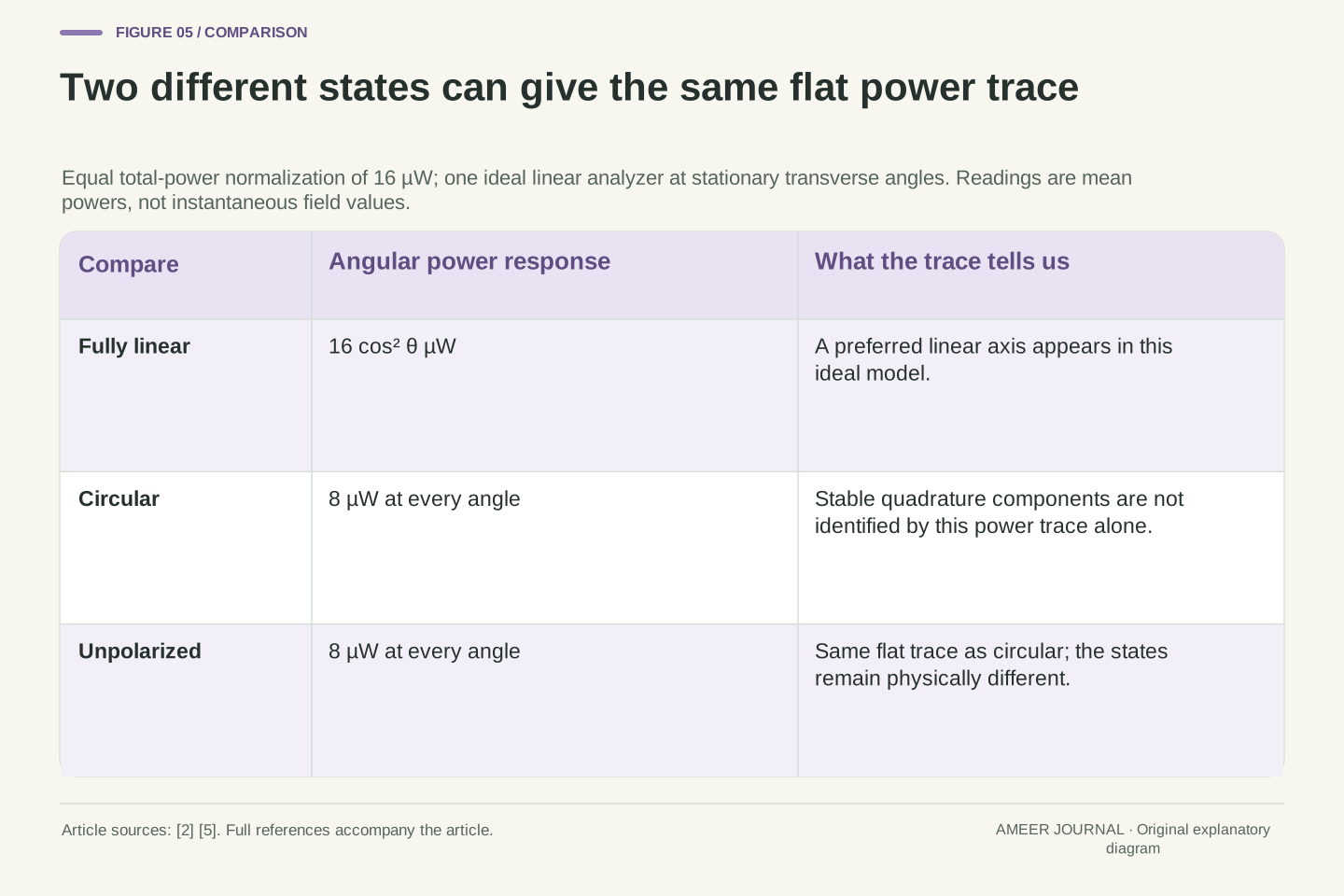
An ideal linear receiving channel takes one projection of that rotating field. Averaged over full cycles, it receives half the total normalized power, whichever transverse angle is chosen. With the same total-power normalization of 16 µW, its mean reading is 8 µW at every angle. Changing the receiver's orientation changes the timing of that projection, but not its mean power.
Unpolarized radiation also gives half its total mean power to an ideal linear channel at every angle. [2] Yet it is not the same state as a circularly polarized wave: it lacks that stable circular relationship between its components. Therefore a flat 8 µW rotation trace could fit either of these two inputs. Power readings alone have left out information needed to distinguish them. Calling a flat trace “unpolarized” without another suitable measurement would turn an incomplete observation into an unsupported identification.
At a fixed position, write a circular field as E(t)=E0[x̂ cos φ+ŷ sin φ], where φ=ωt plus a constant phase. Its squared magnitude is E0² at every instant. Projection onto u(θ) gives E0 cos(φ−θ), whose cycle-averaged square is E0²/2, independent of θ. This derives the half-power response for an ideal linear analyzer without selecting a convention-sensitive circular-handedness name. [2][5]
The comparison uses equal total mean incident power, not equal peak amplitude between a one-component linear sinusoid and a two-component circular field. Those peak-amplitude conventions have different mean-square totals. With a total response normalization of 16 µW, the circular input gives 8 µW per linear channel; a fully aligned linear input gives 16 µW to one channel and zero to its orthogonal partner.
An unpolarized input has no preferred polarization in its averaged second-order statistics and likewise contributes half its total power to any ideal linear analyzer. [2] Its statistical component relationships differ from the coherent quadrature relation of the circular example. Consequently a one-channel mean-power rotation trace cannot distinguish these states. Resolving that ambiguity requires additional polarization-sensitive information, such as appropriately measured intercomponent phase correlations, rather than merely more angles of the same mean-power observable.
A nonzero minimum needs an explanation, not a guess
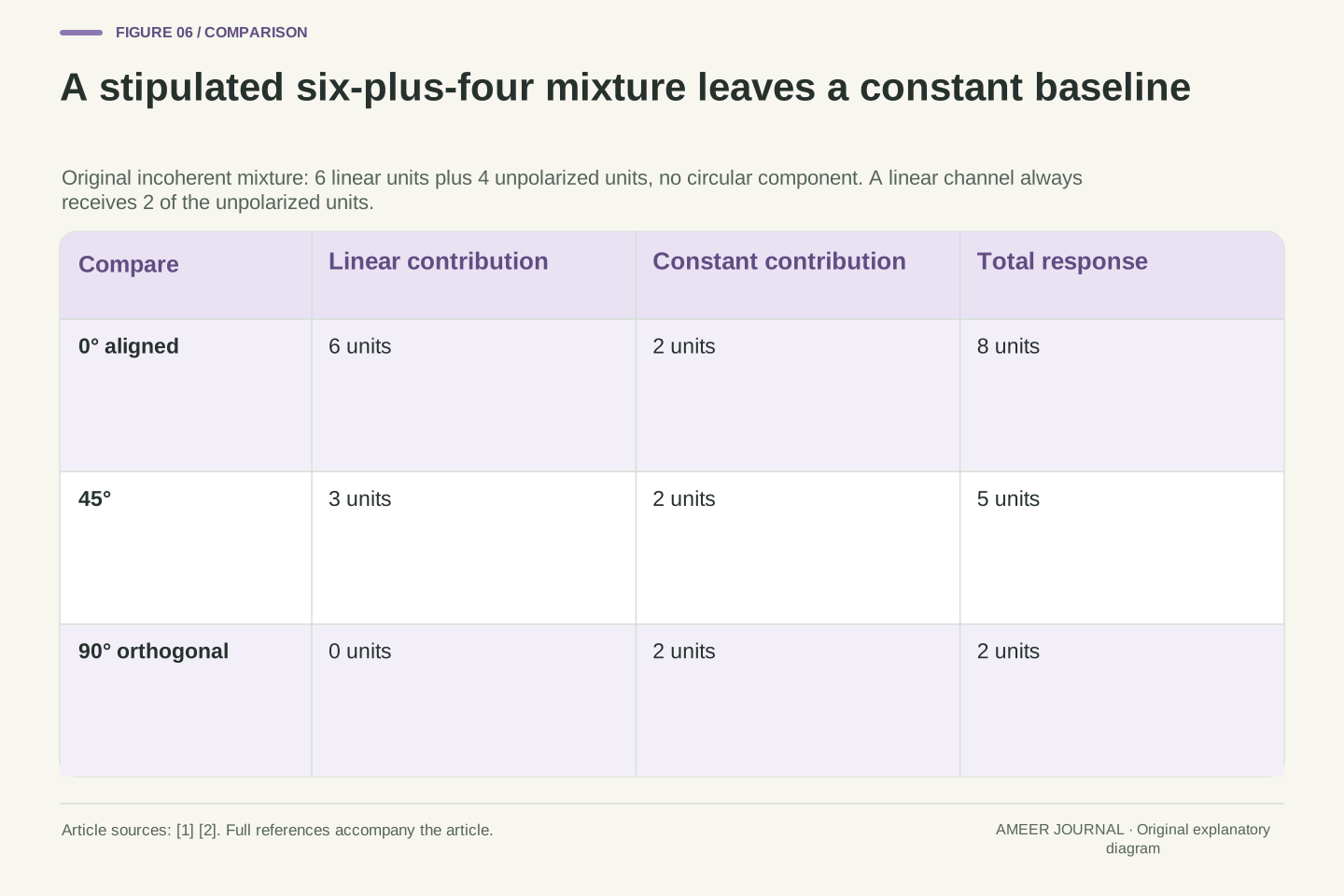
Now stipulate a different hypothetical input: six power units in a linearly polarized component and four in an unpolarized component. The components are independent for the power calculation, so their mean contributions add. We also explicitly say that this example has no circular component. The units are a shared bookkeeping scale, not a new set of measured microwatt readings.
When the receiving axis matches the linear component, it gets all six linear units and half the four unpolarized units: eight in total. At 45 degrees it gets three plus two, making five. At 90 degrees the linear contribution vanishes, leaving two. NRAO describes this combination of an angle-dependent linear response and a constant unpolarized contribution. [1] The minimum is nonzero because the stipulated background still contributes.
The difference between the maximum and minimum is six, while their sum is ten. Their ratio is 6/10, or 60 percent, matching the linearly polarized share we supplied. But the trace alone does not prove that the remaining four units are unpolarized. An independent circular component of four units would also contribute two at every angle. The same readings can therefore fit another physical mixture. The conclusion depends on the stated mixture, not only on the three numbers.
Adopt mutually incoherent components with normalized power Ilin=6 and Iu=4, and explicitly exclude a circular component. Incoherence permits addition of their time-averaged detected powers without a surviving cross term. For the ideal analyzer, R(θ)=Ilin cos² θ+Iu/2=6 cos² θ+2. This follows the partially linearly polarized-source model given by NRAO. [1]
The outputs at 0°, 45° and 90° are 8, 5 and 2 units. The aligned maximum is Rmax=Ilin+Iu/2 and the orthogonal minimum is Rmin=Iu/2. Thus (Rmax−Rmin)/(Rmax+Rmin)=Ilin/(Ilin+Iu)=6/10=0.6. For the stipulated linear-plus-unpolarized mixture, this is both its linearly polarized fraction and its total polarized fraction, because no circular part was included.
That last identification must not be generalized to every measured rotation curve. Replacing the four unpolarized units with an independent four-unit circular component produces the same constant contribution of two units in a linear analyzer. The resulting polarization interpretation differs, although R(θ) is identical. A power-only rotation measurement therefore supports the angular contrast but does not uniquely identify the nature of the constant remainder. Instrumental leakage and unequal calibration would introduce further possibilities outside this ideal example.
Read polarization as one part of a defined measurement
The field arriving at a receiver need not preserve a simple relationship to the transmitter's original field. Scattering can change the polarization information in the returned wave. NASA's explanation of radar polarimetry describes why different transmitted and received polarizations provide complementary information about a surface. [4] Our single unchanging plane wave is therefore a useful starting model, not a complete description of reflections through a building or radar echoes from a landscape.
Radar channel labels make the measurement choice explicit. In HH, the first H names horizontal transmission and the second H horizontal reception. HV instead means horizontal transmission and vertical reception. NASA gives this transmit-then-receive order. [4] The V in HV is not a second frequency or a claim that the echo must be absent. An intervening scene and the receiving instrument have to be considered before interpreting a channel value.
When reading a polarization claim, ask four questions. What field arrives, and what reference axes describe it? What does the receiver select? Is the reported quantity signed voltage, mean power, a ratio or a positive loss? What else was held fixed? Those questions reveal whether the cosine-squared example actually applies. They also keep the result useful: a carefully defined power comparison can explain a receiver response without pretending to identify every polarization state or predict the performance of a whole wireless service.
The incident polarization at a receiver is a property of the received field after propagation and scattering, not simply a label copied from the transmitting antenna. NASA's SAR explanation describes polarization-preserving and depolarizing interactions and the use of multiple transmit/receive channels. [4] Real multipath fields can also combine contributions with different amplitudes, phases and polarization directions. A single real-axis cosine factor must not replace a model of that composite field.
In NASA's radar notation, HH and HV name transmit polarization first and receive polarization second. HV is therefore an H-transmit/V-receive observation, not a frequency label. A nonzero cross-polar return need not contradict the orthogonal null derived for our unchanged linearly polarized incident plane wave: the intervening scene can alter the field presented to the receiver. The notation alone does not determine the scattering mechanism or its strength.
A defensible interpretation specifies the incoming field state, common coordinate frame, receive-channel response, averaging operation and calibration. It then distinguishes a signed projection from its squared-power response, states the reference for any decibel number, and identifies which variables remain fixed. If several physical states give the same observable, retain that ambiguity. The original calculations establish ideal polarization coupling and its inference limits; network capacity, antenna installation and surface classification each require additional evidence and their own models.
Sources & further reading
Explore the references behind this guide. External pages may change after our review.
- 3 Radio Telescopes and Radiometers‣ Essential Radio AstronomyJames J. Condon and Scott M. Ransom / National Radio Astronomy Observatory · Accessed 7 Nov 2026
- 2 Radiation Fundamentals‣ Essential Radio AstronomyJames J. Condon and Scott M. Ransom / National Radio Astronomy Observatory · Accessed 7 Nov 2026
- Wave PolarizationNational Radio Astronomy Observatory / Green Bank Telescope Operations Primer · Accessed 7 Nov 2026
- Polarimetry - NASA ScienceNASA / NASA-ISRO Synthetic Aperture Radar mission · Accessed 7 Nov 2026
- Polarized Fields - MATLAB & SimulinkMathWorks / Phased Array System Toolbox documentation · Accessed 7 Nov 2026
Article updated 7 Nov 2026.
Found something we should revisit?
Good explanations get better with thoughtful feedback.