What you’ll take away
- An ideal accelerometer measures specific force, so support on a table can produce a one-g reading at rest.
- The same full sensor vector can come from stationary tilt or from an upright accelerating device.
- A magnitude close to one g and a stable record do not prove the gravity-only condition.
- A simple low-pass gravity estimate can absorb sustained translational acceleration.
- Calibration corrects channel errors; it does not by itself resolve motion-versus-tilt ambiguity.
Why does a device on a table report acceleration?
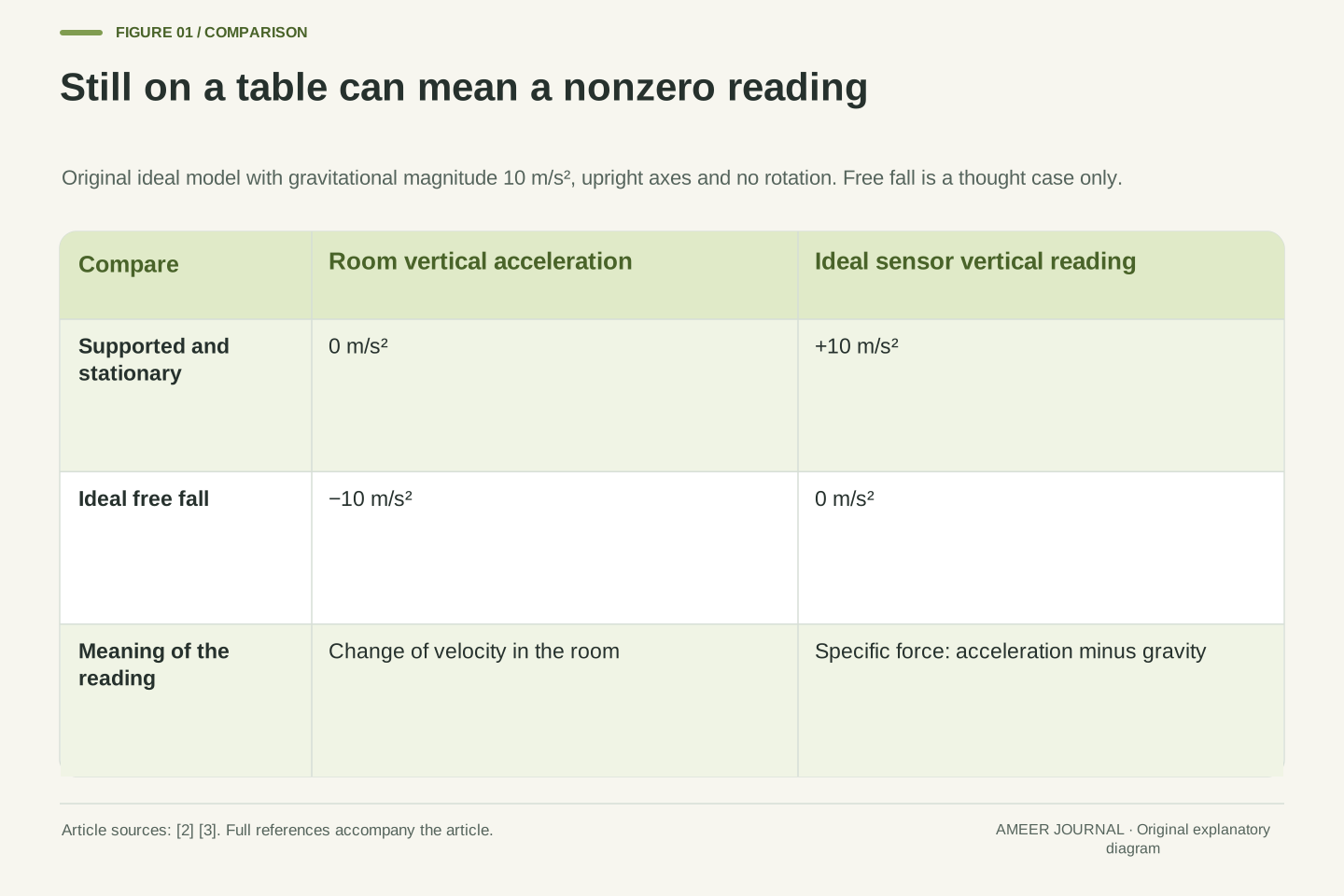
A device can lie still on a table while its accelerometer reports a reading close to one g. That looks like a contradiction if “acceleration” means only a change in the device's speed or direction across the room. The reading answers a different question. An accelerometer responds to the support and other non-gravitational forces acting on it, expressed as force per unit mass. The table keeps the device from falling. With the upward sensor axis correctly identified, that support produces an upward reading even though the device stays in one place. Android and Chrome documentation both describe this stationary-table behavior. [2][3]
The letter g here names the approximate strength of gravity near Earth's surface, commonly about 9.8 metres per second squared. It is not a gram. To make the arithmetic easy to inspect, our imaginary examples use a gravitational magnitude of exactly 10 m/s². Every numerical record below is constructed for explanation, not collected from a phone. We will follow a stationary device, a tilted one and an accelerating one, then ask what their numbers can actually tell us. Free fall appears only as a thought example; there is no reason to drop or throw a device to understand the distinction.
The apparent contradiction comes from conflating world-frame kinematic acceleration with an accelerometer's specific-force output. In the ideal local model used here, a supported stationary sensor has zero kinematic acceleration but nonzero specific force. A freely falling, non-rotating sensor following the gravitational acceleration has zero specific force. The platform documentation gives these limiting cases explicitly, including the positive upward reading for a device supported on a table. [2][3] They are useful sign checks before interpreting any three-axis record.
We use a uniform local gravitational vector of magnitude 10 m/s², a deliberately rounded model value rather than a statement about local gravity or a device's calibration reference. The numerical examples describe an ideal point sensor with known axis conventions. Offsets are absent until the separate calibration example. There are no recorded sensor traces, executed applications or device accuracy results. The aim is to distinguish the observed vector from the assumptions needed to infer tilt or translational acceleration, including a counterexample in which two different physical states produce exactly the same three components.
Keep gravity, motion and the sensor reading separate
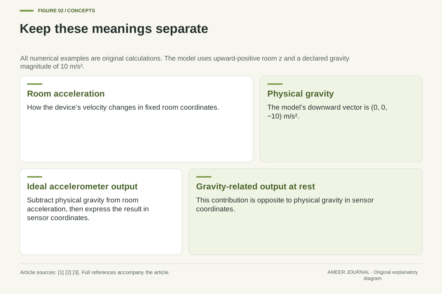
Picture a fixed set of room axes with the positive vertical direction pointing upward. In our model, gravity points downward and has a vertical value of −10. A stationary device has a room acceleration of zero. The ideal accelerometer reading is the device's acceleration minus gravitational acceleration, with both expressed along the same axes. In the vertical direction, zero minus −10 gives +10. The two minus signs explain the positive reading without claiming that the device is moving upward. It is being supported against the fall that gravity would otherwise produce. [2][3]
Now consider ideal free fall without rotation or other forces. The device's downward acceleration is −10 in this model, matching gravity. Subtracting −10 from −10 gives zero. Zero on the accelerometer therefore does not necessarily mean that the device's velocity is unchanging. Conversely, a nonzero reading does not necessarily mean that it is moving across the room. The sensor is useful because it reports this particular physical quantity; the difficulty begins when a label such as “acceleration” hides which quantity is meant. A later software estimate can try to separate motion from the gravity-related part, but that is another step.
Let a be kinematic acceleration in world coordinates and g the gravitational acceleration vector in those coordinates. Let T be an orthogonal transformation mapping world-vector components into sensor-vector components. Define the ideal accelerometer output as f=T(a−g). In this convention g=(0,0,−10) m/s². When T is the identity and a=0, f=(0,0,10). For ideal non-rotating free fall, a=g and f=0. These relationships reproduce the signs in the platform examples. [2][3]
It is useful to define a_s=Ta and q=−Tg, so that f=a_s+q. Here q is the gravity-related contribution to the accelerometer output at rest. It points opposite to physical gravitational acceleration expressed in sensor coordinates. This definition avoids using the same “gravity vector” label for two vectors with opposite signs. All quantities have acceleration units, even when documentation informally describes an acceleration force. The decomposition also shows the information problem: observing f does not independently supply both a_s and q. Assigning the whole observation to q already imposes a condition on motion.
The three channels belong to a coordinate frame
A three-axis sensor reports three signed numbers, usually called x, y and z. They describe components along three directions attached to the sensor or defined by its software interface. They are not automatically east, north and up. Turning a device changes how a fixed room direction is divided among its sensor directions. Android specifies a sensor coordinate system, while web interfaces may distinguish device and screen coordinates. [2][3] Before interpreting a sign, find the positive directions and the coordinate frame in the relevant documentation.
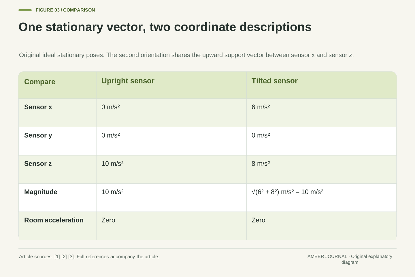
Our first orientation makes sensor z point upward and sensor x sideways. A stationary reading is then (0, 0, 10), with all values in m/s². In a second stationary orientation, the upward support direction is shared between sensor x and sensor z. We choose the reading (6, 0, 8). Its overall size is still 10 because six squared plus eight squared equals one hundred, whose square root is ten. The device has not acquired two separate gravity fields. One vector has different components because the sensor axes point in different directions. Keeping that distinction makes a tilt calculation understandable.
The transformation direction must be stated, because T and its inverse generally give different component signs. Our T maps world components into sensor components. For the tilted example, choose its rows as (0.8,0,0.6), (0,1,0), and (−0.6,0,0.8). This is a proper orthogonal rotation: its rows are mutually perpendicular unit vectors and its determinant is one. It maps the world upward unit vector to (0.6,0,0.8). With a=0, the resulting specific force is f=−Tg=(6,0,8) m/s².
An orthogonal coordinate change preserves vector magnitude, so this static rotation preserves |f|=10 even though two channels become nonzero. Device-axis components should not be treated as world-axis accelerations without the relevant transformation. Platform coordinate conventions and any selected screen-relative remapping are part of the data meaning, not cosmetic display settings. [2][3] A graph can label its vertical plotted channel “z” while the physical sensor z direction is tilted. Reading the graph's axis name alone therefore cannot establish a physical upward direction or justify subtracting a constant from that channel.
A tilt angle needs a condition on motion
If the device is stationary and the sensor is ideal, the reading can reveal how its axes lean relative to vertical. In our x–z example, x reads 6 and z reads 8. The angle between the sensor's positive z direction and upward vertical is about 36.87 degrees. It comes from an angle calculation using the ratio 6 to 8. The exact angle is less useful than the condition that made the calculation valid: we already knew that the device had no room acceleration. Analog Devices explains that inclination sensing assumes that gravity is the only acceleration stimulus contributing to the calculation. [1]
The extra condition matters in ordinary moving systems. A sensor can experience a sustained sideways acceleration as well as support against gravity. Those contributions share the same output channels. A tilt formula will still return a number, but a returned number is not proof that it describes the actual pose. The manufacturer's note specifically warns that additional steady acceleration corrupts an inclination estimate based on gravity alone. [1] Before calling our 36.87-degree result an observed tilt, ask how the no-motion condition was established. A clean display, a stable value and a familiar-looking angle do not establish it by themselves.
For the constructed static x–z orientation, the angle from sensor +z to world upward is θ=atan2(fx,fz)=atan2(6,8)=36.86989765 degrees. The y component is zero and both selected components are positive, so the intended quadrant is explicit. This is an original two-dimensional tilt calculation under a=0. The inclination application note discusses projected gravity, ratios of orthogonal components and the importance of preserving quadrant information. [1] It does not remove the underlying no-confounding-acceleration assumption.
Even in a static setting, gravity provides a vertical reference rather than every aspect of orientation. Two final stationary poses related by a rotation about the world vertical can have the same gravity components when their tilt relative to vertical is otherwise unchanged. Gravity alone therefore does not establish a heading about that vertical. This is a statement about static final poses, not a claim that a sensor located away from a rotation axis would show no acceleration while being moved. The present angle is a specified inclination in a specified plane, not a complete reconstruction of arbitrary three-dimensional motion.
Two different physical states can produce the same vector
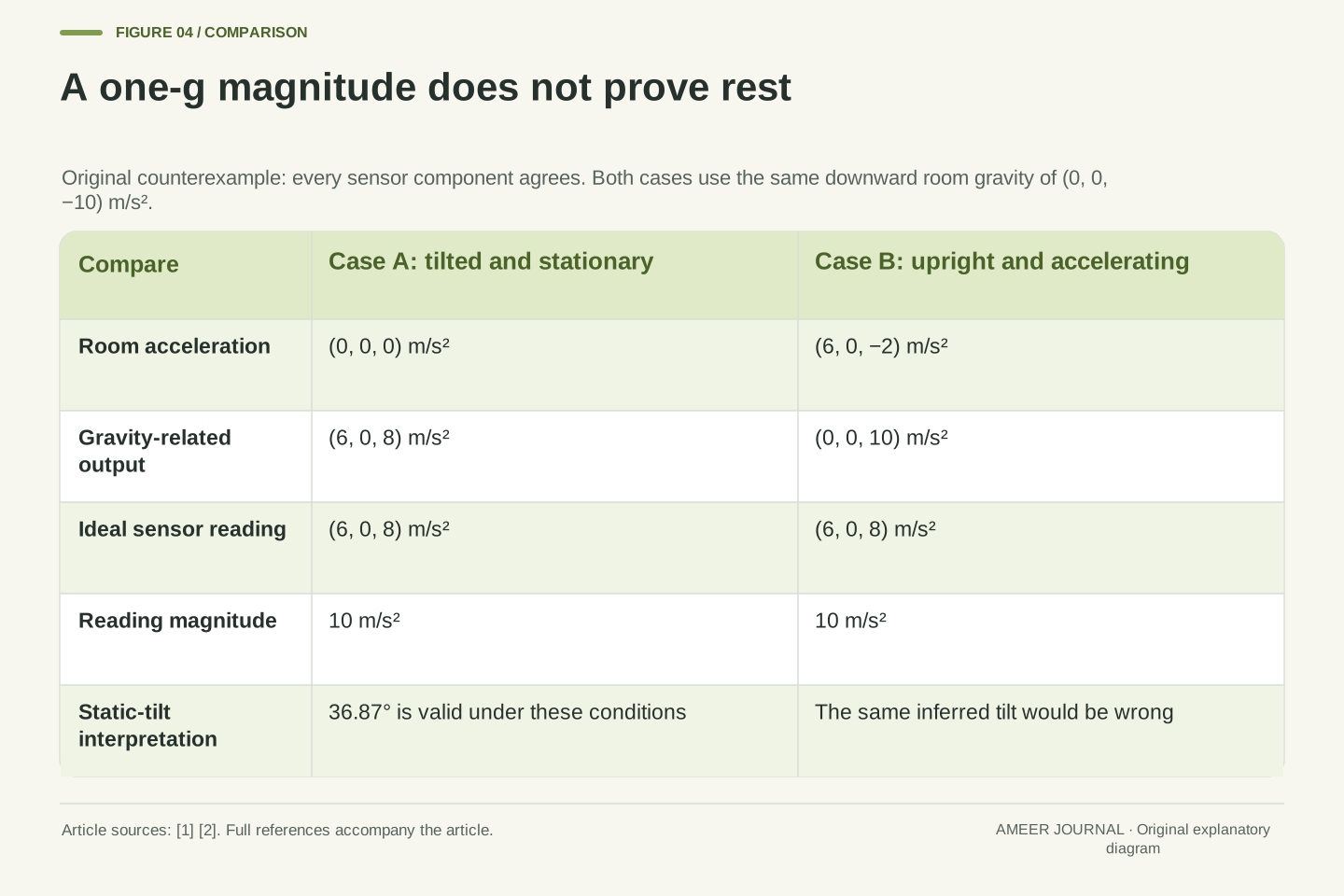
Keep the first explanation of (6, 0, 8): a tilted device resting still. Now consider a second device whose axes remain upright in our room frame. Let its room acceleration be 6 sideways, zero along y and 2 downward, written (6, 0, −2). Subtract gravity, (0, 0, −10), from that room acceleration. The accelerometer output becomes (6, 0, 8), exactly the same three numbers as before. Both calculations use the same units and the same gravity strength. Neither depends on measurement noise.
The second device is not tilted by 36.87 degrees. Its sideways and downward motion changes account for the reading. If the stated acceleration is sustained over a finite interval while the axes remain upright, its output stays constant over that interval. A steady record can therefore have either explanation. The manufacturer's warning about additional constant acceleration is visible here as an exact numerical counterexample. [1] An algorithm that sees only this record must return the same result for both cases, unless it has extra information. It cannot recover a distinction that is absent from its input simply by using a more confident label.
Case A has a=0 and the tilted T defined earlier, giving f=(6,0,8). Case B has T=I and a=(6,0,−2) m/s², so f=a−g=(6,0,8). In A, q=(6,0,8) and a_s=0. In B, q=(0,0,10) and a_s=(6,0,−2). The decomposition changes while the observable vector is identical. Both are valid states of the same ideal model, and the second can persist with fixed orientation and constant acceleration over a finite interval. Over an illustrative two-second interval, Case B changes its world velocity by (12,0,−4) m/s, whereas Case A remains stationary. That difference in velocity history is physically meaningful even though the sensor output is unchanged.
The ambiguity is therefore stronger than a comparison of equal magnitudes or one matching channel. All three components and their constant time histories can agree. An estimator taking only those histories, with the same initial assumptions, has no input feature that separates the two cases. Extra constraints, motion knowledge or another independently informative signal are required for that separation. This is a concrete expression of the application note's warning about DC acceleration contaminating gravity-based inclination. [1] It does not claim that every real motion sequence is indistinguishable, only that accelerometer-only inference cannot be universally unique.
A one-g size is a clue, not a proof of rest
It is tempting to check the overall reading and say, “It is close to one g, so this must be gravity only.” Our two cases show why that shortcut fails. Both give a size of 10 in a model where gravity also has size 10. The tilted stationary case fits the rule, but so does the upright accelerating case. The test accepts a state that violates its intended assumption. A useful check can catch some problems without proving that every accepted record has the desired explanation.
There is a similar problem with treating a constant reading as proof of rest. A constant vector can contain a constant motion-related contribution. A varying vector, meanwhile, might come from changing tilt, changing room acceleration, or both. Analog Devices notes that turning through gravity changes the projections and that filtering affects how quickly the output settles to a new static value. [1] Magnitude, stability and smoothness are useful descriptions of the data. To turn those descriptions into a claim about movement, state the conditions and the additional evidence used. Our example's exact numbers make the logical gap visible before noise complicates it.
The condition |f|≈|g| is not sufficient for a≈0. Our exact counterexample has |f|²=6²+8²=100=|g|² while |a|²=6²+(−2)²=40. In world coordinates, |a−g|²=|g|² implies |a|²−2a·g=0, which admits nonzero a. For Case B, a·g=20 and |a|²=40, so the equality holds exactly. This derived identity explains why the failure is not an artifact of rounding the angle.
A magnitude gate may still be one element of an estimator's decision logic, but it cannot certify the gravity-only condition by itself. Likewise, low variation in f does not establish low translational acceleration. Changing orientation redistributes the gravity contribution, and constant translational acceleration can resemble a changed static orientation. [1] The distinction between a necessary consistency check and a sufficient physical explanation is practical: an accepted sample should retain the assumptions under which it will be used. No threshold or confidence score can turn this particular single-signal counterexample into independent evidence of rest.
Smoothing cannot identify every gravity contribution
A common simple approach treats the slowly changing part of the accelerometer record as gravity-related and subtracts it to estimate motion. Android shows an example that repeatedly blends an old gravity estimate with the new reading. [2] Consider our own calculation with an old estimate (0, 0, 10) and repeated readings (6, 0, 8). At each update, keep 80 percent of the old estimate and add 20 percent of the new reading. After one update, the estimate is (1.2, 0, 9.6). Subtracting it from the reading gives a motion estimate of (4.8, 0, −1.6).
After a second update, the gravity estimate becomes (2.16, 0, 9.28), leaving (3.84, 0, −1.28) as the remainder. With the same input repeated, the estimate gradually approaches (6, 0, 8) and the remainder approaches zero. That is sensible for the tilted stationary case after settling. For the upright accelerating case, however, the method gradually absorbs the sustained motion contribution into what it calls gravity. The smoothing calculation cannot tell the cases apart. It assumes a useful difference in how gravity-related and motion-related parts change over time; it does not discover that difference in every possible record. [1][2]
Use the illustrative recurrence qhat_n=0.8 qhat_(n−1)+0.2 f_n and ahat_n=f_n−qhat_n, initialized with qhat_0=(0,0,10). This has the same simple low-pass structure shown in Android documentation; it is not asserted to be the implementation of every platform gravity or linear-acceleration sensor. [2] For the constant input f_n=(6,0,8), the first two estimates are qhat_1=(1.2,0,9.6) and qhat_2=(2.16,0,9.28). The corresponding residuals are (4.8,0,−1.6) and (3.84,0,−1.28).
More generally, qhat_n=f+0.8^n(qhat_0−f), so ahat_n=0.8^n(f−qhat_0) tends to zero. The true Case B sensor-frame kinematic acceleration remains (6,0,−2), however. A constant translational component is passed into the low-pass estimate together with the gravity contribution. The filter also introduces a settling response after genuine reorientation, as the manufacturer warns. [1] These are model limitations, not arithmetic defects. The example specifies update counts without a sampling interval, so it provides no settling time in seconds. Choosing a different blend changes the response rate without resolving the identical-input ambiguity.
Calibration fixes a different kind of mistake
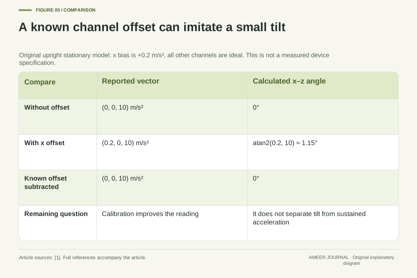
So far, the sensor itself has been ideal. Now imagine a known horizontal-axis offset: x reports 0.2 m/s² too high while the other channels are exact. An upright stationary device that should read (0, 0, 10) instead reports (0.2, 0, 10). A gravity-only tilt calculation interprets that small sideways value as about 1.15 degrees of lean. This angle comes from the ratio 0.2 to 10. The device has not leaned; the output has an added offset. Analog Devices explains why offsets and unequal axis sensitivities can create inclination errors. [1]
If the offset is independently known, subtracting 0.2 from x restores the ideal reading in this example. That correction addresses a measurement error. It does not solve the earlier ambiguity between a perfect sensor that is tilted and a perfect sensor that is accelerating. Both problems can appear in a real system, so they need separate reasoning. Calibration should also match the quantity being calibrated: shifting a displayed angle by one constant is not generally equivalent to correcting the sensor channels before calculating angles. The manufacturer's guidance applies offset and sensitivity corrections to the acceleration values first. [1]
Introduce an additive sensor-frame bias b=(0.2,0,0) m/s² and otherwise retain ideal scale and alignment. With true upright specific force f=(0,0,10), the measured vector is m=f+b=(0.2,0,10). The apparent x–z inclination is atan2(0.2,10)=1.14576284 degrees. Subtracting the independently known b before angle calculation restores zero inclination in this toy model. The value 0.2 is an invented example, not a sensor specification, uncertainty bound or measured calibration result.
The application note separates offset error from relative sensitivity error and recommends correcting the acceleration outputs before computing inclination. [1] A more general measurement model would include scale factors, cross-axis effects and noise, but adding those terms is unnecessary to demonstrate this offset mechanism. Correcting b improves the accuracy of f; it does not supply a separate observation of a_s or q. Consequently, even perfect calibration leaves the two-state counterexample intact. This is the distinction between inaccurate observation of a physical quantity and non-unique inference of two physical quantities from an accurate observation of their sum.
Read the name of the output before subtracting anything
A device or app may offer an accelerometer value, a gravity estimate and a linear-acceleration value. Those names should lead you to different expectations. Android describes the accelerometer output as including the gravity-related contribution, and linear acceleration as excluding it. At rest, its gravity output should match its accelerometer output. [2] Chrome documentation likewise distinguishes an accelerometer's supported one-g reading from the near-zero linear-acceleration reading expected at rest. [3] Three numbers labelled “acceleration” therefore need more context than their units alone.
In our sign convention, an upright stationary accelerometer reads upward +10, and the gravity-related part to subtract is also upward +10. The physical gravitational acceleration in the room is downward −10. Mixing those two meanings of “gravity” would produce the wrong subtraction. A software estimate can use information beyond a single accelerometer, and some exposed sensor quantities are calculated or fused rather than direct hardware outputs. [2][3] Its documentation should explain what it represents. Neither the output name nor the presence of three decimal places guarantees a particular accuracy, availability or motion-separation method on every device.
Android's documented conceptual relation is linear acceleration equals accelerometer acceleration minus its gravity contribution. Its gravity output uses the accelerometer coordinate system and should match the accelerometer at rest. [2] In our notation that subtraction is a_s=f−q, where q=−Tg. It is not f−Tg. The latter would add the downward physical-gravity vector's opposite a second time and yield 20 m/s² vertically for the upright stationary toy case. Explicitly naming the vector convention prevents an API label from reversing the physical sign.
Reported gravity and linear acceleration may involve software estimation or sensor fusion, while the underlying accelerometer measures a different physical signal. The platform sources distinguish low-level and derived sensor interfaces. [2][3] This article does not infer a specific fusion algorithm from an API name, nor assume identical implementations across hardware. Interpret units, frame, calibration state, timestamps and quantity definition together. If a supplied linear-acceleration signal already has a gravity contribution removed, subtracting that contribution again is a different operation. The provenance of the value matters as much as the numerical transformation applied to it.
Here, “raw accelerometer” is shorthand for the gravity-inclusive accelerometer quantity, not a promise of untouched electrical samples or absent factory correction. Android separately documents an uncalibrated accelerometer type without bias compensation. [2] Those are different distinctions: whether gravity is included describes the physical quantity, while whether bias compensation is applied describes processing of that quantity. A gravity-inclusive output can still be calibrated, and a gravity-removed output can still have estimation errors. Keeping those two labels independent makes an exported record much easier to interpret than using “raw” as a catch-all description.
What would make a sensor explanation convincing?
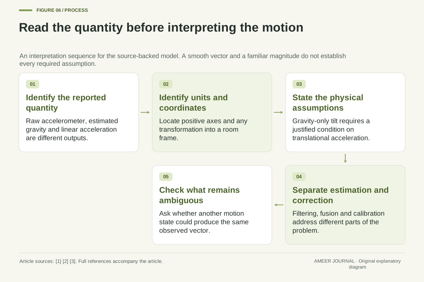
Start with the question the reading is supposed to answer. If it is about tilt, establish why motion-related acceleration can be ignored or explain what other information separates it. If it is about room movement, find how the gravity contribution and coordinate frame are handled. Then check a simple reference case: with our upright stationary model, the raw ideal reading is (0, 0, 10), while the ideal linear-acceleration result is zero. A sign or output-label mistake often becomes visible in that comparison before a complicated record is interpreted.
Return to the original surprise. One g on a table is consistent with support against gravity. A one-g-sized reading elsewhere does not, by itself, prove that the device is stationary or reveal a unique tilt. Our exact pair of (6, 0, 8) readings demonstrates why. Smoothing can produce a useful estimate under suitable assumptions; calibration can correct known channel errors; additional information can constrain motion. Each has a different job. A convincing explanation states which job was done and preserves the remaining uncertainty instead of asking one sensor vector to answer more questions than it contains.
A defensible interpretation records the measured quantity, units and coordinate transformation before choosing an inference model. The reference equations are f=T(a−g), q=−Tg and a_s=f−q. The static inclination calculation additionally requires a=0 or a justified approximation to it. A magnitude check, a low-pass recurrence and a bias correction operate at different stages of that reasoning. Their outputs should not be substituted for independent evidence that the static condition holds. The source guidance on inclination assumptions, sensor semantics and filtering supports these distinctions. [1][2][3]
The original examples provide several separate checks: the rest and free-fall signs; the rotated (6,0,8) gravity contribution; the identical upright accelerating state; the exact one-g magnitude counterexample; the recurrence converging to a wrong decomposition for sustained acceleration; and the small apparent angle caused by a known offset. Together they identify what is observed and what must be assumed. None requires a claim about a particular phone's performance. The useful result is a reproducible explanation of why an accelerometer can be functioning correctly while an apparently reasonable interpretation of its values is still underdetermined.
Sources & further reading
Explore the references behind this guide. External pages may change after our review.
- AN-1057: Using an Accelerometer for Inclination Sensing | Analog DevicesChristopher J. Fisher / Analog Devices · Accessed 6 Nov 2026
- Motion sensors | Sensors and location | Android DevelopersAndroid Developers / Google · Accessed 6 Nov 2026
- Sensors for the web | Capabilities | Chrome for DevelopersChrome for Developers / Google · Accessed 6 Nov 2026
Article updated 6 Nov 2026.
Found something we should revisit?
Good explanations get better with thoughtful feedback.