What you’ll take away
- A fresh digital sample can describe a sensing element that has not yet reached the intended medium temperature.
- A first-order time constant marks about 63.2% of a temperature change, not complete settling.
- Specify the allowed residual and initial difference before calculating a waiting time.
- Compare response fractions, models and physical conditions before comparing quoted seconds.
- A stable reading can retain error from other thermal paths, self-heating or the reporting chain.
A fresh number can describe a sensor that is still catching up
Imagine a digital thermometer showing a new number every second. The surrounding temperature suddenly rises, and the display begins climbing. The numbers arrive promptly, yet they remain below the new temperature for some time. There is no contradiction. The electronics can report the sensing element's temperature quickly while that element is still warming. A digital result does not remove the need for heat to move into or out of the sensor. Manufacturers discuss thermal response separately from the conversion that turns a sensor signal into a readable value. [1][2][4]
The useful question is therefore more precise than “How fast is this thermometer?” Ask which part is fast: taking an electronic reading, delivering it to the screen, or physically approaching the temperature you want to measure. Those parts can have different answers. We will follow an invented sensor through a mathematical temperature change, using no real thermometer experiment. The example explains measurement timing; it is not a guide to judging body temperature, food safety or hazardous equipment. Its numbers belong to the assumptions stated below, not to a product sold under a particular brand. Keep the target temperature and the sensor temperature separate from the start.
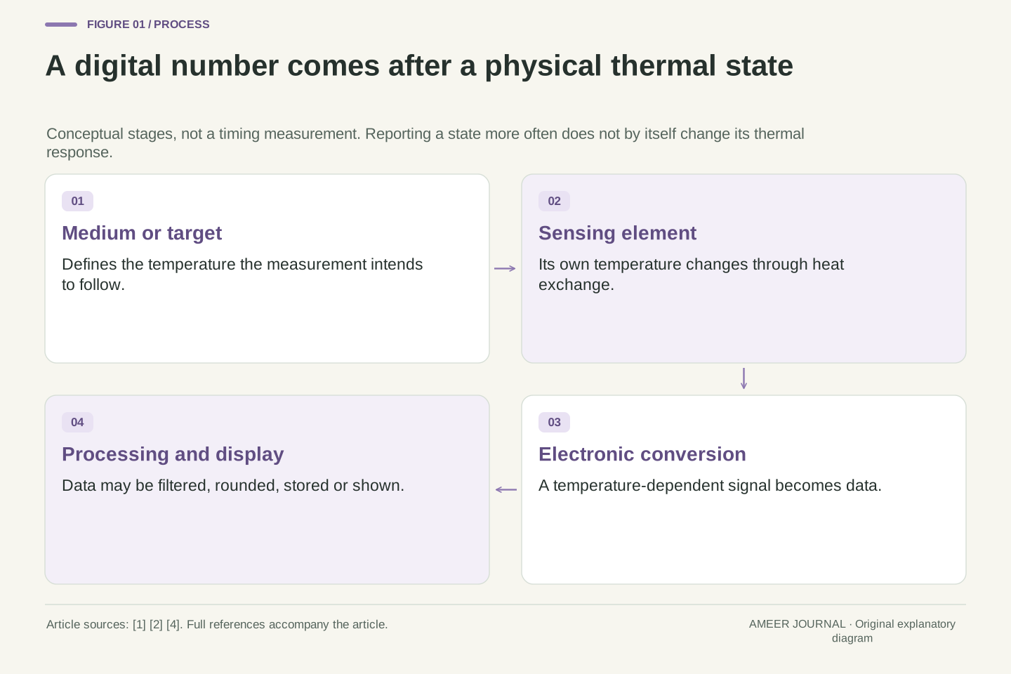
A temperature measurement chain contains a thermal state as well as an electrical representation. The sensor element responds to heat exchange with its surroundings; a transducer and acquisition system then encode a temperature-dependent property. Increasing the rate at which that representation is read does not, by itself, reduce the thermal inertia of the element and package. A fresh sample may be an accurate representation of the sensor's present state while differing from the temperature of the intended medium. The manufacturer's first-order response explanation and its separate description of digital conversion support this distinction. [1][4]
The reader question here concerns transient tracking, not the relative quality of analog and digital products. Define the intended measurand before evaluating the output: ambient air, a board, a contacted surface and the sensing die are different physical objects. A system can encode one reliably without establishing that it equals another. We use a deliberately idealized temperature step to isolate thermal lag, then restore the installation and self-heating qualifications that the idealization leaves out. Every numerical trajectory is calculated from that model; there are no reported measurements, hardware benchmarks or clinical conclusions. The distinction also prevents display resolution from being mistaken for a dynamic accuracy guarantee.
Separate warming, conversion and reporting
First comes the physical response: the sensing part exchanges heat and changes temperature. Second comes the electronic measurement: the instrument converts its temperature-dependent signal into data. Third comes reporting: software may store, smooth, round or display that data. These are connected stages, but their times are not interchangeable. A one-second display update does not say that the sensing element reaches a new surrounding temperature in one second. A fast conversion also cannot recover a final temperature that the element has not yet reached merely by printing more decimal places. [2][4]
To make the distinction concrete, suppose our later model is read instantly once per second. Its first reading after the change would be about 20.33°C, even though the surroundings have already reached 40°C. The screen has new information; that information says the sensor has only started warming. Reading ten times as often would reveal more points along the same assumed warming curve. It would not change the curve under these assumptions. Real instruments may add averaging, delays or measurement-related heating, so the simple “more samples, same curve” statement depends on holding the physical system and its power use unchanged. TE's discussion of update rate and self-heating is one reason that qualification matters. [2]
Distinguish thermal response, conversion timing and output timing. Conversion can have its own acquisition or integration interval; a communication or display schedule can be slower still. Optional filtering transforms the available sequence rather than changing the already completed heat exchange. Treating a reported sample as an instantaneous thermal state is an explicit simplification in our calculation. It is not a description of every converter or every application's timestamp semantics. Digital-output sensor architectures can include a temperature-dependent generator, an ADC and encoding circuitry, illustrating that reporting is downstream of sensing. [4]
For an ideal sampler with negligible conversion and transport delay, samples at integer seconds are simply T(0), T(1), T(2) and so forth. The model below gives T(1)=20.33057°C. Sampling at ten samples per second instead produces additional evaluations of the same continuous function, provided sampling does not alter power or thermal coupling. That proviso has practical meaning: measurement current can cause self-heating, and a device's operating duty cycle may affect it. [2] Faster reporting is therefore neither proof of faster thermal response nor inherently thermally neutral. To compare two records, identify whether a timestamp represents acquisition, the end of an averaging interval, transmission or display; the timestamp label alone cannot resolve that choice.
Give the warming model a clear starting point
Our invented sensor begins at 20°C, matching its surroundings. At time zero, the surroundings jump to 40°C and remain there. We suppose the sensor behaves as one uniformly warm object, with one constant response time scale of 60 seconds. We also leave out self-heating, other heat sources and any electronic delay or measurement error. These choices produce a simple example in which the only difference between the sensor and its surroundings comes from its gradual thermal response.
This is called a first-order model. The sensor approaches the new temperature quickly at first and more slowly as the gap shrinks. The time scale, usually written as the Greek letter tau, tells us how quickly that remaining gap decreases. Analog Devices describes this kind of thermal response with a first-order model and a time constant. Its handbook connects the response to thermal resistance and thermal mass. [1][4] That connection is useful: the sensor has some capacity to store thermal energy, and its thermal connection controls how readily energy moves. A protective package or a different environment can change those properties. The model is a chosen approximation, not a promise that every real probe follows one perfect curve.
Use a lumped, isothermal sensing body with heat capacity Cth and a single thermal resistance Rth to a prescribed medium temperature Ta. With constant positive parameters, no self-heating and no competing heat path, its energy balance is Cth dT/dt=(Ta−T)/Rth. The time constant is τ=Rth Cth. Thermal resistance has units K/W and heat capacity J/K, giving τ in seconds. This is the thermal analogue of a single resistance-capacitance response, consistent with the manufacturer's explanatory approximation. [1][4] Spatial gradients and multiple thermal masses can require a richer model.
Set T(0)=20°C, Ta=40°C for all t≥0, and τ=60 s. The solution is T(t)=40−20 exp(−t/60), with time in seconds. Temperatures here may be expressed in Celsius because the energy balance and exponential response involve temperature differences. A 20°C interval equals a 20 K interval; no absolute-temperature ratio is being used. At t=0 the equation returns 20°C, and its long-time limit is 40°C. Those two checks establish that the initial condition and final boundary condition are represented correctly. They do not validate the approximation for a real installation, which would require appropriate evidence about that sensor and its thermal surroundings.
Sixty-three percent means part of the change
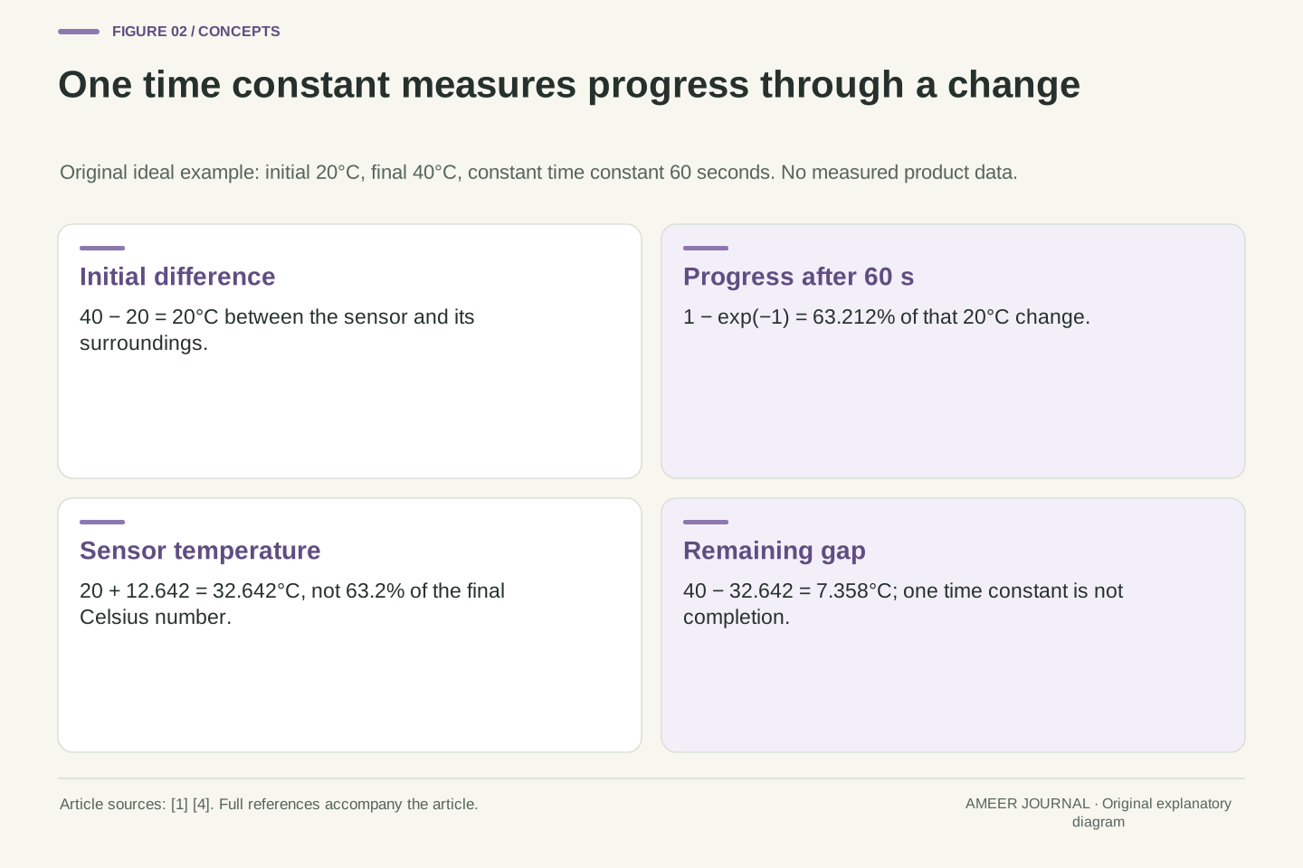
After one time constant, this first-order sensor has completed about 63.2% of the temperature change. The change is 40−20=20°C. About 63.2% of that interval is 12.64°C, so the sensor reaches about 32.64°C after 60 seconds. It is still about 7.36°C below its surroundings. The time constant therefore does not mean “time until the thermometer is finished.” It marks a particular point on the approach to the final temperature. [1][4]
The phrase “63.2% of the final temperature” is easy to misread when a short specification uses it. Multiplying 40°C by 0.632 would miss the starting point of this example. Instead, find the starting value, find the change, apply the fraction to that change, and add the result to the start. This also works for cooling: the change then has a negative sign. It should not depend on whether you label the same temperatures in Celsius or kelvin. The meaningful fraction describes how far the sensor has travelled between its initial and final states, rather than a percentage of a temperature scale's chosen zero. That small wording distinction prevents a large arithmetic mistake.
Define the normalized step response as f(t)=[T(t)−T0]/[Ta−T0], for a nonzero step. In the stated model, f(t)=1−exp(−t/τ). At t=τ, f=1−exp(−1)=0.63212056. For a 20°C step, the increase is 12.642411°C and T(60)=32.642411°C. Equivalently, the residual is exp(−1)=0.36787944 of the initial difference. These are fractions of a difference, not ratios to the absolute Celsius endpoint. [1][4]
An affine change of temperature scale leaves f unchanged because the zero offset cancels in both differences. That is a useful consistency check on any percentage-response interpretation. If a calculation changes the physical response merely by converting Celsius to kelvin, it has probably divided absolute readings where it needed differences. For a downward step, numerator and denominator are both negative during the response, so the same positive fraction still describes progress toward the endpoint. A zero-size step has no defined normalized fraction, although the constant-temperature solution remains valid. The sources' shorthand about a percentage of the final value is interpreted here through this explicit step definition; it is not reproduced as an absolute-temperature formula.
Follow the shrinking gap through five time constants
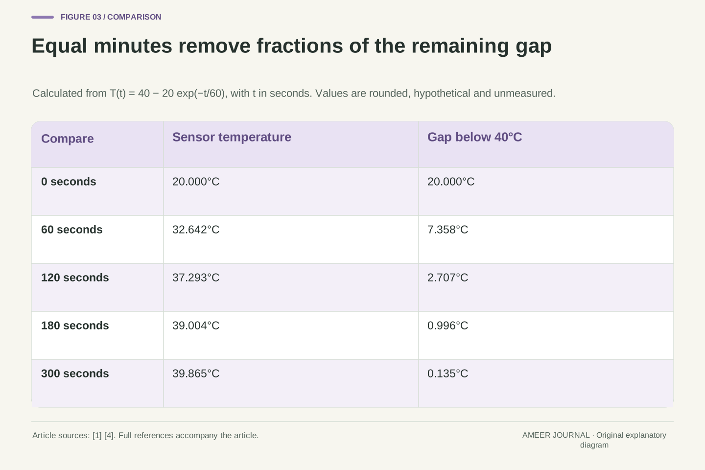
At the start, our sensor reads 20°C. After 60 seconds it reaches about 32.64°C. After 120 seconds it reaches about 37.29°C, and after 180 seconds it reaches about 39.00°C. At 300 seconds, five time constants after the change, it reaches about 39.87°C. These values come from the same equation. They are not measurements from five different products and do not describe five separate settings.
Notice that equal time intervals do not add equal amounts of temperature. The first minute adds about 12.64°C, while the second adds about 4.65°C. The sensor has less of a gap left to close. A mistaken straight-line prediction that adds another 12.64°C every minute would soon take it above the unchanged surroundings, which this model does not allow. After three time constants, roughly 95% of the original change is complete; after five, roughly 99.3% is complete. The remaining difference is small, but it is not exactly zero. [1][3][4] Whether that difference matters depends on the purpose and tolerance of the measurement. “It has almost stopped changing” and “it is close enough for this task” require different evidence.
Evaluating the original model at 0, 60, 120, 180 and 300 s gives 20, 32.642411, 37.293294, 39.004259 and 39.865241°C respectively. Corresponding residuals relative to the 40°C boundary are 20, 7.357589, 2.706706, 0.995741 and 0.134759°C. Each additional time constant multiplies the residual by exp(−1). Thus equal intervals remove a fixed fraction of the remaining difference, not a fixed number of degrees. The reported decimals show the calculation, not the attainable resolution of a physical sensor.
The derivative is dT/dt=(20/60)exp(−t/60) °C/s, positive and decreasing for this upward step. It begins at one-third of a degree per second and tends toward zero. The resulting trajectory is monotonic and cannot overshoot its constant boundary under the stated assumptions. At 3τ the response fraction is 0.95021293; at 5τ it is 0.99326205. The common approximately 95% association with three time constants also appears in the NPL paper's abstract. [3] An actual record that overshoots, oscillates or follows several slopes is not explained by this single ideal model alone; it calls for examination of the boundary conditions, acquisition processing or additional physical dynamics, rather than silently redefining the time constant.
Choose the acceptable difference before choosing a waiting time
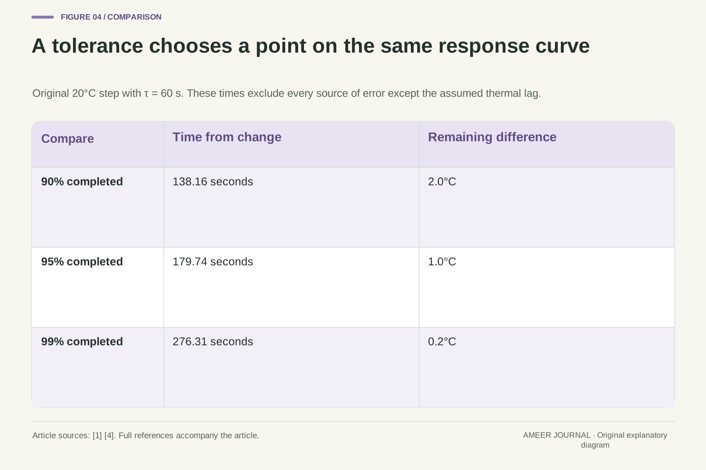
Suppose the question is when the invented sensor comes within 0.2°C of the 40°C surroundings. Starting 20°C away, it must reduce the gap to one-hundredth of its original size. That means completing 99% of the change. In this example, the calculated time is about 276.31 seconds, a little over four and a half minutes. A 60-second time constant alone would not have answered that question.
Different targets give different times. Completing 90% of the change takes about 138.16 seconds and leaves a 2°C gap. Completing 95% takes about 179.74 seconds and leaves a 1°C gap. Completing 99% takes about 276.31 seconds and leaves a 0.2°C gap. These are alternative tolerances for one model, not three accuracy ratings. [1][4] The size of the initial change also matters when the tolerance is stated in degrees. With the same assumed time constant but only a 2°C initial gap, reaching a 0.2°C gap would require 90%, rather than 99%, completion. Do not turn any of these times into a general instruction for a real thermometer: its actual response, installation and allowed error have to be established separately.
For fractional completion f between zero and one, solve 1−exp(−t/τ)=f to obtain tf=−τ ln(1−f). With τ=60 s, t90=138.155106 s, t95=179.743936 s and t99=276.310211 s. The logarithm is natural. For a positive allowed residual ε smaller than the initial magnitude |ΔT|, the equivalent expression is t=τ ln(|ΔT|/ε). Our |ΔT|=20°C and ε=0.2°C yield ln(100) time constants. The ratio is dimensionless.
This calculation answers a residual-error question within a specified model, not a total uncertainty question. It excludes calibration error, noise, quantization and non-target thermal paths. If ε is already at least the initial gap, the initial state satisfies that tolerance; the logarithmic expression should not be interpreted as a required negative waiting time. For ε=0, exact agreement is reached only as a limiting value in this ideal exponential model. A measured display can show the rounded endpoint sooner, because finite resolution can hide a nonzero residual. Consequently a displayed 40.0°C is not, by itself, evidence of mathematically zero lag or zero measurement error. The response criterion should be set before interpreting an apparently settled reading.
A larger number of seconds can describe the faster sensor
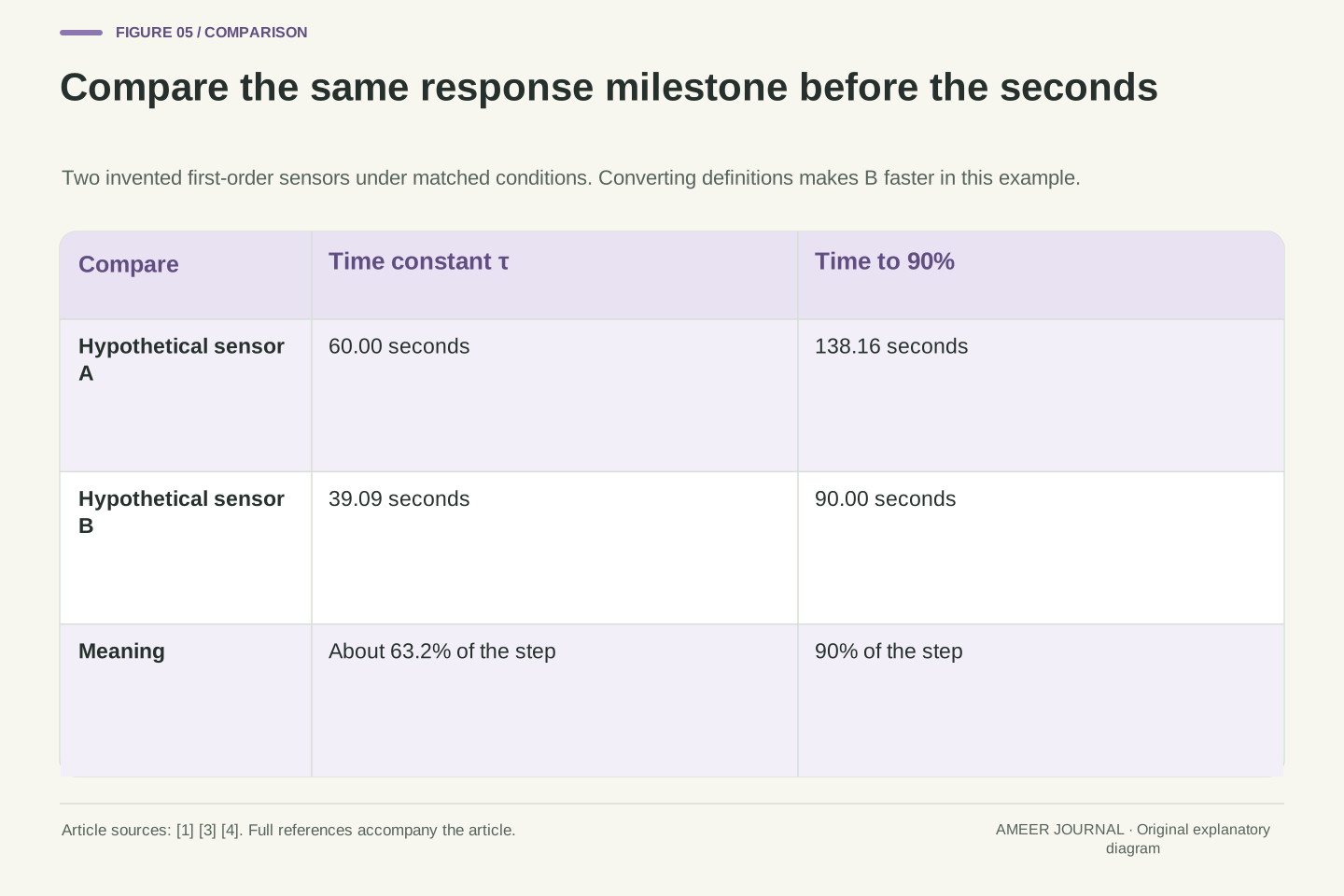
Consider two more clearly hypothetical descriptions. Sensor A has a 60-second time constant. Sensor B takes 90 seconds to complete 90% of a step. It is tempting to compare 60 with 90 and call A faster. That compares two different milestones. The first number refers to about 63.2% completion; the second refers to 90% completion. A fair comparison first needs the same milestone and the same measurement conditions.
Under the same first-order assumptions, A needs about 138.16 seconds to complete 90% of its change. B needs 90 seconds because that is how its description was defined. B is therefore faster in this particular comparison, even though its quoted number was larger. Alternatively, B's time constant works out to about 39.09 seconds, which can be compared directly with A's 60 seconds. [1][4] This example does not rank real products. It shows why a response-time statement needs a percentage, a definition and a description of the conditions. A bare “response: 60 seconds” leaves too much unanswered to support a confident comparison. Check whether an accompanying graph, footnote or test description supplies the missing meaning.
Let A have τA=60 s and B have t90,B=90 s. For the same single-pole response convention, t90=τ ln(10). Thus t90,A=138.155106 s, while τB=90/ln(10)=39.086503 s. Comparing t90 values identifies B as faster under these hypothetical matched conditions. Comparing time constants gives the same result. A comparison of 60 s with 90 s without converting the definitions would reverse the conclusion for no physical reason.
The conversion is conditional on a first-order representation. A multi-stage thermal system can have a response shape for which one percentage-crossing time does not determine every other crossing time. Its reported t90 should then be used as defined, or interpreted through a supported response model, rather than forced into a single τ. Likewise, two measurements made in different media or at different airflow rates may not establish a product ranking for either intended installation. [3][4] Name both the endpoint criterion and the test environment before converting. The calculation here is a consistency exercise: it demonstrates what identical model assumptions allow, while keeping the response fraction separate from the seconds used to reach it.
The surrounding medium is part of the response
A sensor does not warm in isolation from its surroundings. Its size, package, contact and surrounding medium affect how heat reaches the sensing part. TE identifies thermal mass and thermal conductivity as contributors to step response. The Analog Devices handbook shows that airflow changes the response of one specified sensor and mounting arrangement. [2][4] A time measured under moving air therefore should not be silently reused for still air or a different mounting setup.
Research on meteorological thermometers illustrates the same issue in another setting. The public abstract of a 2020 paper held by the National Physical Laboratory identifies ventilation rate and sensor diameter as important factors in its response study. [3] That is evidence for why conditions matter, rather than a current specification for your device. A protective enclosure may change the thermal situation; contact with a board may make the board part of what the sensor follows. First decide which object's temperature you intend to know. Then look for response evidence under conditions that actually relate to that object. “Faster in one published test” does not automatically mean faster in every use, especially when the route by which heat enters the sensor has changed.
The effective resistance and heat capacity in a lumped model depend on the physical realization. Medium properties, flow, contact, package dimensions and attached material can alter the response. The manufacturer's handbook discusses die and case contributions and presents an airflow-dependent time constant for a particular package and board arrangement. [4] Those numerical conditions are source-specific; they are not parameters of our τ=60 s toy. TE separately associates step response with both sensor and medium thermal properties. [2]
The NPL repository exposes the abstract of Burt and de Podesta's 2020 meteorological sensor paper. It reports that ventilation and diameter are important contributors in its experimental and theoretical study. [3] We rely on that scoped result, not on an unread full paper or an inferred current meteorological requirement. For a real comparison, the sensor identity is only part of the record: mounting, exposure, medium and relevant flow conditions define the thermal coupling as well. A changing environment also differs from the ideal permanent step used here. One may need a time-dependent boundary condition, several coupled thermal states or other validated dynamics. Reusing a time constant without its conditions can hide that model change even when the part number remains identical.
A stable reading can still belong to the wrong thermal balance
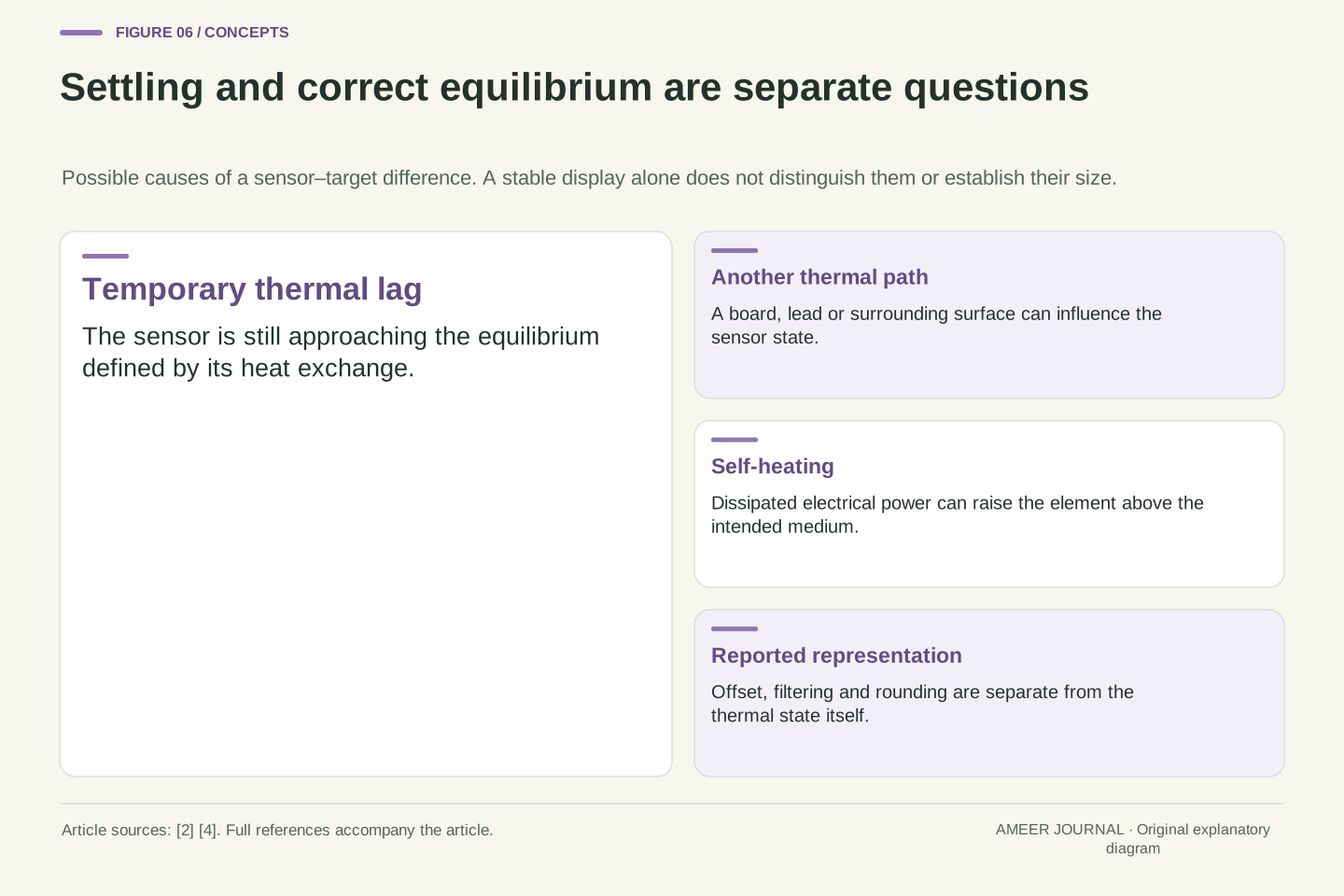
Waiting addresses thermal lag only when the eventual sensor temperature is the one you want. A warm circuit board, a cooler wire connection or heat produced by measurement current can affect that eventual temperature. TE warns about unintended heat sources and self-heating. The Analog Devices handbook also discusses wiring as a thermal path and power dissipation as a source of temperature rise. [2][4] The sensor may eventually stop changing while remaining different from the intended surroundings.
This is why a steady number does not prove that all errors have disappeared. In our ideal example, the only heat connection leads to the 40°C medium, so 40°C is the limiting value. Add another continuing heat input and the original equation no longer describes the whole situation. More waiting cannot remove a heat source that remains present. Nor can extra display digits show which physical object established the sensor's temperature. A useful diagnosis separates a temporary tracking difference from a persistent difference caused by the measurement arrangement. Both may appear as a gap between two readings, but they do not have the same cause or the same remedy. Any practical correction needs evidence about the actual system.
The no-power, one-path model has a well-defined equilibrium T=Ta. With constant self-heating power P and the same single thermal resistance, its energy balance becomes Cth dT/dt=(Ta−T)/Rth+P, giving the equilibrium T∞=Ta+P Rth. This elementary extension explains why a persistent input can create an offset even after the transient decays. The handbook explicitly relates dissipated power and thermal resistance to sensor die-temperature rise; TE notes measurement-current self-heating in digital sensors as well. [2][4]
Additional thermal connections require their own terms and boundary temperatures. A lead or board can transport heat toward or away from the element, so the sign cannot be assumed without the surrounding temperatures. A stable sensor state may then reflect several boundaries rather than the intended target alone. Separately, electrical offset, scale error or rounding can affect the reported value without being thermal-state errors. Those mechanisms should not be merged into a single “slow sensor” explanation. A stationary display establishes only limited evidence about time variation at its reporting resolution; it does not identify the heat paths or establish traceable agreement with the measurand. The original exponential example intentionally excluded these effects so that its residual had one unambiguous cause.
Read a response claim as a complete measurement statement
A useful response statement says what was measured, what changed and what counted as reaching the target. For our example, that statement is: an ideal first-order sensor starts in equilibrium at 20°C, its only surrounding medium steps to a constant 40°C, its time constant is 60 seconds, and its instantaneous, error-free output is calculated. Under those assumptions it reaches 99% of the change after about 276.31 seconds. Each part contributes information; removing the percentage or the initial gap changes what the timing number tells you.
For an actual specification, look for the corresponding physical and electronic details: the sensing target, medium, mounting, response fraction and acquisition conditions. Sources may place those details in separate notes, so read them together. [1][2][3][4] If only the update rate is supplied, you can describe how often new data is reported, but you cannot calculate thermal settling from that number alone. If only a thermal response is supplied, you still need to know how the application records or displays it. This gives a practical answer to the original puzzle: frequent updates can faithfully reveal a slow approach. The right interpretation comes from identifying what is changing, which stage produced the number and how close the task requires the sensor to be.
A reproducible response interpretation binds a time metric to a model and conditions: initial equilibrium, imposed boundary change, sensor construction and mounting, medium and flow, response criterion, plus the acquisition operation applied to the thermal state. Our analytical record specifies all of these through deliberate simplification. Its result is a calculation with known assumptions, whereas a real specification must supply relevant measured or otherwise validated evidence. A source's product-specific response figure should remain attached to its documented test conditions. [1][2][3][4]
Keep the final inference proportional to the available information. Update frequency alone determines neither τ nor a total error bound. A percentage response time alone does not prove a single-pole model. A small visible slope alone does not establish correct equilibrium. Conversely, a disagreement shortly after a change need not show a calibration fault if the two quantities being compared have different thermal dynamics. Before choosing a correction, identify the physical state, the reported representation and the error criterion. In the worked example those distinctions turn “a quick thermometer seems slow” into a precise statement: the assumed output is immediate, but the sensor's 20°C thermal difference decays with a 60-second time constant.
Sources & further reading
Explore the references behind this guide. External pages may change after our review.
- What is the thermal response time constant of the DS1922L? - FAQs - Sensors Library - EngineerZoneAnalog Devices / EngineerZone official FAQ · Accessed 6 Nov 2026
- Digital vs Analog Sensors: Considerations | TE ConnectivityTE Connectivity · Accessed 6 Nov 2026
- Response times of meteorological air temperature sensors | NPL PublicationsNational Physical Laboratory / Stephen Burt and Michael de Podesta · Accessed 6 Nov 2026
- Sensor Signal Conditioning: Section 7, Temperature SensorsAnalog Devices · Accessed 6 Nov 2026
Article updated 6 Nov 2026.
Found something we should revisit?
Good explanations get better with thoughtful feedback.