What you’ll take away
- A display can accurately report the connected voltage while the meter input changes that voltage from its earlier value.
- The input resistance forms a parallel branch whose effect depends on the source resistance as well as the meter.
- In the original model, a one-percent loading limit requires an input resistance at least 99 times the effective output resistance.
- Two simultaneous meter inputs must be combined before recalculating the circuit; their individual voltage drops cannot simply be added.
- One loaded reading does not uniquely determine both the unloaded voltage and the source resistance.
A correct display can describe a circuit that the meter has changed
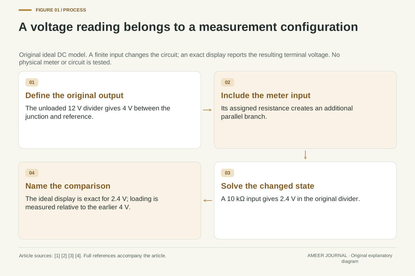
An imaginary voltmeter displays 2.4 volts. Its display is exactly right for the voltage between its terminals, yet the same circuit had 4 volts between those points before the meter was present. There is no contradiction. The instrument became part of the circuit and changed the quantity being observed. Checking the display against the voltage that exists now answers a different question from asking how much the measurement arrangement changed the earlier voltage.
OpenStax explains that a voltmeter is placed across the two points whose potential difference is of interest, and that its resistance matters to the disturbance it introduces [1]. NI and NJIT likewise describe the effect of a finite input resistance [3][4]. We will follow one invented, steady direct-current circuit on paper, with exact resistances and an ideal display. The example is a calculation, not an assembly activity or a test of a commercial meter. Its deliberately conspicuous loading makes three quantities easy to separate: the voltage before the meter, the voltage after it, and the indicated value.
A voltage measurement has an intended measurand, a measurement configuration and an indication. In the original model here, the unconnected output is 4 V, the output after adding the meter input is 2.4 V, and an ideal indication reports that loaded terminal voltage exactly. Indication error relative to the loaded state is therefore zero by construction, while the change relative to the unloaded state is nonzero. The reference state must accompany any statement that the reading is correct.
OpenStax places a voltmeter in parallel with the potential difference being measured [1]. NI and NJIT discuss its finite input resistance and the resulting influence on the circuit [3][4]. Our construction uses an ideal 12 V source, positive linear resistors, steady DC conditions and an exact indicator with a specified parallel input resistance. There is no physical meter, simulation package, calibration or uncertainty estimate. Within those boundaries, elementary network equations let us separate loading, indication and inference about the original circuit without assigning a product an unsupported accuracy claim.
First calculate the voltage before adding a measurement branch
Start with a 12 V source and two resistors in one series path. The upper resistor is 20 kilo-ohms and the lower resistor is 10 kilo-ohms. A kilo-ohm is one thousand ohms. The output is the junction between the resistors, measured relative to the lower end of the 10 kilo-ohm resistor. Treat that lower end as zero volts. No other path leaves the junction in this first state. Naming both points matters because voltage describes a difference between points, not a quantity belonging to a loose wire alone.
Series resistances add, and the same current passes through both components in this arrangement [2]. The total is 30 kilo-ohms, so the current is 12 divided by 30,000, or 0.0004 ampere. That is 0.4 milliampere. Across the lower 10,000 ohms, this current produces 4 V. The upper resistor accounts for the remaining 8 V, giving the source's full 12 V together. These are assigned ideal values. They establish the undisturbed reference against which we will compare a second, explicitly changed circuit.
Let the source be Vs = 12 V, the upper resistance Ru = 20 kΩ and the lower resistance Rd = 10 kΩ. Define the lower endpoint as the reference node and V as the junction potential relative to it. With no external output branch, the two resistors are in series. Ohm's law and the series-current relation give I0 = Vs/(Ru+Rd) = 0.4 mA and V0 = I0 Rd = 4 V [2]. Here V0 denotes the unloaded output of this particular divider, not the source voltage.
The corresponding upper drop is I0 Ru = 8 V, so the two drops sum to 12 V. This baseline uses an ideal source with no separately assigned source resistance; Ru is a real element of the hypothetical divider rather than a hidden instrument parameter. The output terminal is open only with respect to an added external branch: current still flows through the original divider. Keeping that distinction explicit prevents “unloaded” from being misread as zero current everywhere in the network.
The input resistance creates another path across the lower resistor
Now give the imaginary voltmeter an input resistance of 10 kilo-ohms. Its ideal display observes the voltage without introducing any additional effect beyond that assigned resistance. When represented across the output and the reference point, the meter input shares both endpoints with the lower resistor. It is therefore a parallel branch, not another resistor in the original series chain [1][2]. This 10 kilo-ohm value is chosen to make the arithmetic visible. It is not a claim about the usual resistance of a digital multimeter.
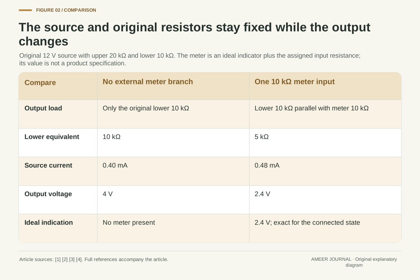
The original lower resistor has not vanished, and its resistance has not changed. Instead, current arriving at the junction can now take either of two equal 10 kilo-ohm paths. Two equal parallel resistances have an equivalent resistance half as large: 5 kilo-ohms. The source consequently sees the upper 20 kilo-ohms followed by this 5 kilo-ohm equivalent. The network has changed even though the source and original resistors have retained their values. We must solve this new network before deciding what voltage the meter will display.
Model the meter as an ideal voltage indicator with a finite resistance Rm connected between the output node and reference. Set Rm = 10 kΩ for the first case. Since Rd and Rm share both nodes, their conductances add: 1/Rp = 1/Rd + 1/Rm. Thus Rp = Rd Rm/(Rd+Rm) = 5 kΩ [2]. The ideal indicator adds no current beyond the stated Rm. NJIT uses a real-instrument resistance alongside an ideal instrument to explain this distinction [4].
The upper resistor is in series with the parallel combination, so the total resistance seen by the ideal source becomes Ru+Rp = 25 kΩ. It would be incorrect to place Rm in series with Rd or to replace Rd by Rm while discarding the existing lower branch. The meter changes connectivity at the output. The assigned resistance is an illustrative input parameter, not a commercial specification, and the calculation intentionally excludes capacitance, leakage variation and range-dependent behavior. Those effects would require a different input model rather than a correction to this parallel-resistance formula.
The meter current is not the same as the increase in source current
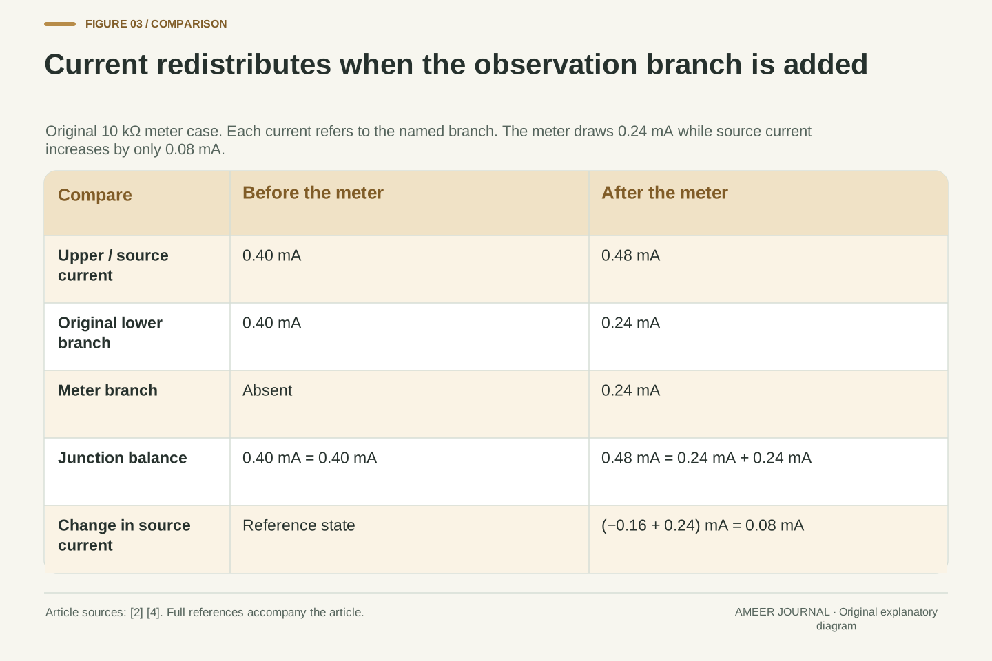
With a total resistance of 25 kilo-ohms, the source now supplies 12 divided by 25,000, or 0.48 milliampere. The voltage across the lower parallel combination is 0.48 milliampere times 5 kilo-ohms: 2.4 V. Both parallel branches share that voltage. The lower resistor carries 0.24 milliampere, and the meter carries another 0.24 milliampere. Their sum is the 0.48 milliampere through the upper resistor, consistent with current conservation at the junction [2]. The ideal display therefore reports 2.4 V correctly.
Notice the difference between the meter's current and the source's increase. The meter carries 0.24 milliampere, but the source increased only from 0.40 to 0.48 milliampere, a change of 0.08. The original lower branch fell from 0.40 to 0.24 milliampere because its voltage fell. Its decrease accounts for the rest. Simply adding the meter current to the old source current would miss this redistribution. Relative to the original 4 V, the new voltage is 1.6 V lower, a 40 percent reduction. That is loading, not a display mistake.
For the loaded network, Is = 12/25 kΩ = 0.48 mA and V = Is Rp = 2.4 V. The branch currents are Id = V/Rd = 0.24 mA and Im = V/Rm = 0.24 mA, with Is = Id+Im. The upper drop is 9.6 V and the lower drop is 2.4 V, again summing to the ideal source's 12 V. Both current and voltage balances agree with the series/parallel relations in OpenStax [2].
The change in source current is ΔIs = 0.48−0.40 = 0.08 mA, whereas Im = 0.24 mA. These differ because ΔId = 0.24−0.40 = −0.16 mA, so ΔIs = ΔId+Im. The loaded network must be solved as a whole rather than treated as the old currents plus an independent meter current. With the unloaded output as denominator, (V0−V)/V0 = (4−2.4)/4 = 0.4. The ideal indicator's error relative to V remains zero. This separates two comparisons that an unqualified “40 percent measurement error” would blur.
Summarize the output with its unloaded voltage and output resistance
Instead of recalculating the lower parallel pair for every meter, we can summarize how this divider responds at its output. Two numbers are needed: the unloaded 4 V and an effective output resistance. For this particular ideal divider, that resistance is the upper resistance times the lower resistance, divided by their sum. It is 20 × 10 ÷ 30, or 6⅔ kilo-ohms. The next section uses that quantity to compare different meter inputs without changing the original divider.
The resulting voltage is the unloaded voltage multiplied by the meter resistance divided by the sum of the meter resistance and the effective output resistance. With a 10 kilo-ohm input, that is 4 × 10 ÷ (10 + 6⅔) = 2.4 V. This is an algebraic summary of the terminal relationship, derived from the same current balance used above [2]. It does not say the original 12 V source has become a 4 V source inside the circuit. The simplified description preserves what the added load sees; it does not reproduce every internal current.
Write the output-node balance as (Vs−V)/Ru = V/Rd + V/Rm. Rearranging gives V = Vs Rd Rm/(Ru Rd + Ru Rm + Rd Rm). Define V0 = Vs Rd/(Ru+Rd) and Ro = Ru Rd/(Ru+Rd). Substituting these definitions yields V = V0 Rm/(Ro+Rm). This source-equivalent form follows directly from the specified resistor relations [2]; NJIT separately identifies output resistance as a source property relevant to loading [4]. For our divider, Ro = 20/3 kΩ.
The equivalent describes the output terminal voltage-current relation for this linear model. It does not identify Ro with the lower 10 kΩ resistor alone, nor does it preserve the divider's internal source-current accounting. For example, the equivalent source's series current is the external load current, while the original 12 V source also supplies the lower divider branch. Thus terminal equivalence cannot be used to substitute one network's internal source power for the other's. The reduction is useful precisely when its preserved boundary is stated.
Compare input resistances while keeping the source model fixed
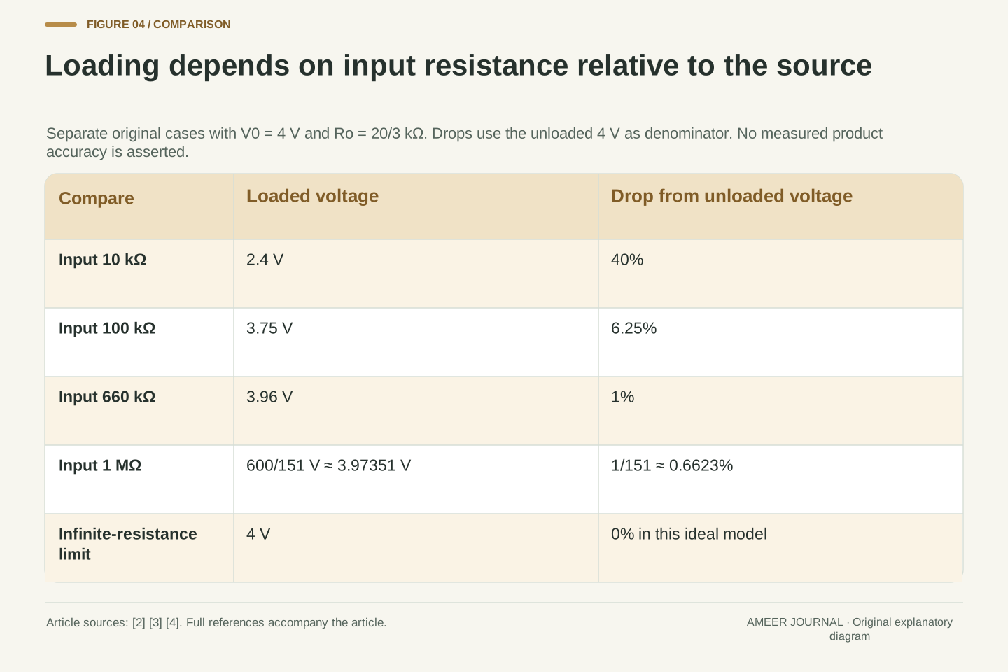
Keep the same 12 V source and 20/10 kilo-ohm divider. A meter input of 100 kilo-ohms gives an output of 3.75 V. The reduction from the unloaded 4 V is then 0.25 V, or 6.25 percent. A 1 mega-ohm input, equal to 1,000 kilo-ohms, gives about 3.97351 V, only about 0.6623 percent below 4 V. These are separate model cases, each with one meter input present. They are not a sequence of readings collected from an instrument.
For this fixed circuit, increasing the input resistance makes the added branch draw less current and brings the output closer to the unloaded value. The ideal limit of infinite input resistance returns 4 V. NI describes infinite input resistance as an ideal and discusses finite and selectable input resistance in real instruments [3]. That does not establish one universal value for every instrument or range. The comparison here concerns loading alone. More display digits, by themselves, would not change the resistance of the branch or restore the earlier circuit voltage.
Use V = 4 Rm/(Rm+20/3) with resistances expressed consistently in kΩ. Rm = 10 kΩ yields 2.4 V; Rm = 100 kΩ yields 15/4 V = 3.75 V; and Rm = 1000 kΩ yields 600/151 V ≈ 3.9735099 V. Their relative drops from V0 are respectively 2/5, 1/16 and 1/151. These cases change only Rm and retain the original source and divider. The values are exact algebra followed by clearly marked rounding, not measured meter performance.
For positive V0 and Ro in this construction, the loading drop decreases monotonically as Rm increases and tends to zero as Rm tends to infinity. NI's discussion supports the finite-input loading mechanism and notes selectable input configurations [3]. It does not justify treating all ranges or measurement tasks as equivalent. Indication resolution is also a separate parameter: our display was stipulated exact from the outset, so its precision cannot explain the difference between 2.4 V and 4 V. That difference comes entirely from the modeled terminal load.
A one-percent loading limit refers to the source resistance
Suppose our paper requirement is to keep the loading reduction at or below one percent of the original voltage. The denominator is the unloaded 4 V, so the allowed drop is 0.04 V and the connected output must be at least 3.96 V. Solving the model gives a minimum meter resistance of 660 kilo-ohms. At exactly that value, the voltage is 3.96 V and the drop is exactly one percent. This condition covers only the change caused by the assigned input resistance.
The ratio behind the result is instructive. The meter resistance must be at least 99 times the divider's effective output resistance of 6⅔ kilo-ohms. Being ten times that output resistance is not enough for a one-percent limit: it leaves a drop of one part in eleven, about 9.09 percent. The comparison is with the effective output resistance, not automatically with either physical resistor. An overall measurement uncertainty would also need other information that this model has not supplied. Our exact display assumption does not turn the loading calculation into a complete instrument specification.
Define the relative loading drop e = (V0−V)/V0 for V0>0. Substituting the terminal relation gives e = Ro/(Rm+Ro). For a required bound 0<ε<1, e≤ε is equivalent to Rm≥Ro(1/ε−1). With ε = 0.01 and Ro = 20/3 kΩ, the threshold is 99Ro = 660 kΩ. The boundary voltage is V0(1−ε) = 3.96 V. All percentages therefore have an explicit unloaded-voltage denominator.
At Rm = 10Ro, e = 1/11 ≈ 9.0909 percent and V = 40/11 V ≈ 3.63636 V. The familiar-looking ten-to-one ratio cannot be substituted for the derived 99-to-one requirement. This inequality is exact only for the declared positive, purely resistive DC model. It budgets loading, not source variation, resistance tolerances, offsets, noise, gain error or a real meter's calibration uncertainty. The distinction is substantive: a model can satisfy its loading inequality while additional unmodeled error terms remain unknown rather than zero.
The same unloaded voltage does not imply the same loading behavior
Now create a separate divider with both resistors ten times larger: 200 kilo-ohms above the output and 100 kilo-ohms below it. Keep the source at 12 V. The ratio of the resistances is unchanged, so the unloaded output remains 4 V. However, its effective output resistance is now 66⅔ kilo-ohms, also ten times larger. A single 100 kilo-ohm meter input gives 2.4 V on this divider, even though that same input gave 3.75 V on the original one.
The source current before adding a meter also differs. The original unloaded divider carries 400 microamperes, while the scaled divider carries 40 microamperes. A microampere is one millionth of an ampere. Equal output voltage did not make the two networks identical. NJIT's discussion of instrument influence relates the disturbance to circuit resistance as well as instrument resistance [4]. Our comparison makes that dependency numerical: the input resistance has to be considered alongside the source that drives it. An isolated 4 V label leaves out information needed to predict the connected reading.
Scale both divider resistances by a factor s = 10 while retaining Vs. The unloaded ratio Rd/(Ru+Rd) is unchanged, so V0 remains 4 V. Meanwhile Ro becomes sRuRd/(Ru+Rd) = 200/3 kΩ. With the same Rm = 100 kΩ, the output is V = 4×100/(100+200/3) = 2.4 V. The original divider with that input instead gives 3.75 V. Input resistance alone therefore does not fix the loading fraction.
The unloaded current scales inversely with s: 12/30 kΩ = 400 µA for the original divider and 12/300 kΩ = 40 µA for the scaled one. The current and output-resistance changes are consequences of the assigned ideal resistances, not claims about the quality or power efficiency of products. NJIT's instrument-loading discussion provides the relevant circuit-resistance context [4]. The preserved property under scaling is the unloaded voltage ratio; the load-dependent terminal relationship changes. Reporting the unloaded voltage without Ro would conceal that difference even though both baseline voltages are correct.
Two agreeing displays can share the same changed voltage
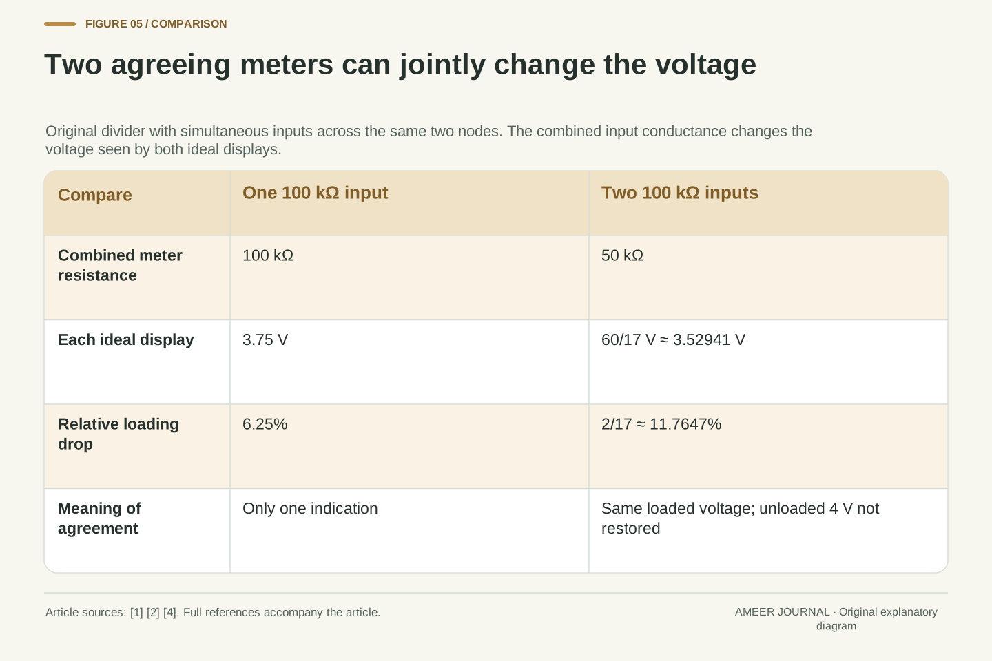
Return to the original divider and represent two 100 kilo-ohm meter inputs across its output at the same time. Together those inputs form a 50 kilo-ohm load. Recalculating the whole network gives about 3.52941 V, and both ideal displays show that same value because they share the same two endpoints. Their agreement confirms the equality of their indicated terminal voltages in this model. It does not establish that the voltage stayed at the unloaded 4 V.
With only one 100 kilo-ohm input, the drop was 0.25 V. It would be tempting to subtract that twice and predict 3.50 V for two meters, but the actual model result is 60/17 V, about 3.52941 V. Each input's current depends on the new shared voltage, so the second configuration cannot be calculated by adding two independent one-meter drops. Parallel conductances add; the voltage must then be solved again [2]. A second observer can therefore change the state being compared while still agreeing perfectly with the first observer's display.
Two simultaneous Rm = 100 kΩ inputs have combined resistance 50 kΩ. With Ro = 20/3 kΩ, their common output is V = 4×50/(50+20/3) = 60/17 V. Each meter carries (60/17)/100 kΩ = 3/85 mA. The original lower resistor carries 6/17 mA, and the source carries 36/85 mA. Adding the lower current and both meter currents gives that same source current, independently checking the node balance [2].
The relative drop is (4−60/17)/4 = 2/17 ≈ 11.7647 percent. Adding two separate one-meter drops would instead predict 12.5 percent and 3.5 V, because each 0.25 V drop was calculated for a different network with only one input. The correct aggregation adds input conductances before solving for V. Both ideal indications agree exactly at the jointly loaded state. Neither agreement nor zero indication error establishes equality with the unloaded reference; the measurement configuration remains part of the quantity being compared.
One loaded reading does not uniquely reveal the earlier voltage
If the input resistance and the effective output resistance are both known within our model, the loaded reading can be used to calculate the unloaded voltage. Multiply the reading by one plus the output resistance divided by the meter resistance. For the original 10 kilo-ohm input and 2.4 V reading, the factor is one plus 6⅔ divided by 10. The result is 4 V. This is a conditional reconstruction from known parameters, not something the displayed number reveals on its own.
To see the missing information, consider another hypothetical source with an unloaded voltage of 3 V and an output resistance of 2.5 kilo-ohms. The same 10 kilo-ohm meter would again show 2.4 V: 3 × 10 ÷ 12.5. Thus one identical reading is compatible with at least two different unloaded voltages. A correction formula cannot decide which source description applies unless that description is established separately. The issue is not insufficient decimal places. It is that the observation contains less information than the pair of unknown source quantities.
Rearranging the terminal relation gives V0 = V(1+Ro/Rm). This recovers V0 only conditionally on the model and known Ro and Rm. Case A uses V0 = 4 V, Ro = 20/3 kΩ and Rm = 10 kΩ, producing V = 2.4 V. Case B uses V0 = 3 V, Ro = 2.5 kΩ and the same Rm, also producing V = 3×10/12.5 = 2.4 V. The two cases are an original algebraic counterexample, not observations from two physical sources.
One loaded voltage with known Rm therefore does not uniquely identify both V0 and Ro. The terminal equation constrains their relationship but leaves more than one compatible pair. This is separate from display accuracy: the indication can be exact in both cases while the inferred unloaded voltage remains ambiguous. Additional justified information would be needed to identify the relevant source model. No two-load procedure is carried out here, and no correction is claimed for a nonlinear or time-varying source to which the derived linear relation may not apply.
Keep the reference state and input model beside the voltage
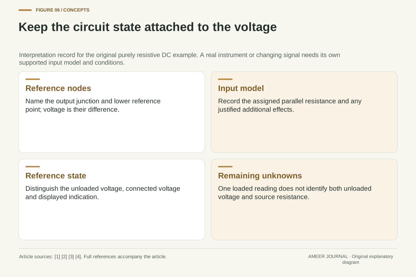
A useful interpretation records which two points define the voltage, what circuit was present, and what the instrument input adds between those points. It also states whether the desired answer concerns the connected state or the earlier unloaded state. In our example the first answer is 2.4 V and the second is 4 V. Both are correct for their named configurations. Calling either number simply the true voltage would remove the condition that explains why they differ.
The paper model treats the input as a fixed resistance and waits for no changing signal. NJIT notes that instrument impedance can involve capacitance or inductance as well as resistance, while NI discusses different input configurations [3][4]. Those are reasons to retain the model boundary when interpreting real specifications. Our result establishes neither dynamic behavior nor a universally best measurement range. It establishes a narrower, useful point: an accurate indication of the connected circuit can coexist with a substantial change from the circuit you meant to observe. The input's effect and the display's accuracy need separate evidence.
An inspectable loading calculation specifies the reference nodes, unloaded network, source assumptions, instrument input model and intended measurand. It distinguishes V0, the loaded V and the indication. For the original 10 kΩ input, the derived values are V0 = 4 V, V = 2.4 V and indication = 2.4 V. The loading fraction is 40 percent relative to V0, while indication error relative to V is stipulated zero. These statements remain compatible because their reference quantities differ.
The resistive DC reduction is not a general instrument-impedance model. NJIT explicitly allows capacitive and inductive components, and NI describes finite and selectable input behavior [3][4]. Frequency dependence, settling, noise, component uncertainty, protection and actual range specifications are not resolved by the present numbers. Nor does increasing Rm in this fixed model establish the best choice for every task. What survives the example is the reasoning sequence: define the desired state, include the observation branch, solve the changed network, and state which comparison the resulting voltage supports.
Sources & further reading
Explore the references behind this guide. External pages may change after our review.
- 10.4 Electrical Measuring Instruments - University Physics Volume 2 | OpenStaxOpenStax / Rice University · Accessed 7 Nov 2026
- 10.2 Resistors in Series and Parallel - University Physics Volume 2 | OpenStaxOpenStax / Rice University · Accessed 7 Nov 2026
- Digital Multimeter (DMM) Measurement Fundamentals - NINI · Accessed 7 Nov 2026
- ECE 291 - Lab 4: Internal impedance of instruments, influence of instruments on circuitsNew Jersey Institute of Technology, ECE Undergraduate Laboratories · Accessed 7 Nov 2026
Article updated 7 Nov 2026.
Found something we should revisit?
Good explanations get better with thoughtful feedback.