Imagine comparing two telescope designs. The second has twice the opening diameter, but it observes light with four times the wavelength. Which produces the narrower image of a distant point of light? The larger opening helps, yet the longer wavelength pushes the diffraction pattern in the other direction. In the simple circular-opening model used here, the second pattern has twice the angular radius to its first dark ring. NASA’s Hubble-and-Webb comparison describes the same underlying trade-off: observing longer wavelengths requires a wider mirror to retain a comparable level of angular detail [3].

We will use three invented designs to separate three questions: how wide a point-source pattern is on the sky, how much light the opening collects, and how large the image becomes at the detector. These are paper calculations, not measurements of Hubble, Webb or another observatory. Each design has an ideal clear circular opening, uniform illumination, one wavelength, accurate focus and no image motion. Those assumptions let us change diameter and wavelength independently. Later, we will check what changes when the image is enlarged without changing the opening at all.

An aperture comparison needs both diameter D and wavelength λ. For the ideal circular pupil considered here, the first-minimum angular radius follows θ≈1.22λ/D. Doubling D while increasing λ fourfold therefore doubles θ. The resulting larger angle means a broader diffraction scale, even though the collecting area has increased. NASA’s conceptual comparison of Hubble and Webb explicitly connects longer observing wavelength with the larger aperture needed for comparable angular detail [3]. Its resolving-power language must be distinguished from the resolution angle used here, for which smaller is finer.

The original model assumes monochromatic far-field point sources, a uniformly illuminated, unobscured circular pupil, paraxial image geometry and an otherwise ideal stationary optical system. Wavelength and diameter use compatible length units. The coefficient 1.22 is the familiar rounded circular-pupil value, not a universal constant for every telescope geometry. Our calculations compare conditional optical quantities; they do not simulate an intensity image, observe a source or reproduce an actual instrument’s performance. Keeping angular scale, collecting area and focal-plane scale separate is the central purpose of the three-design construction.

A geometric sketch often shows parallel light rays meeting at a single point. Wave optics gives a fuller picture. Through an ideal circular opening, light from one distant point forms a bright central region surrounded by rings. Light from different parts of the opening combines in ways that strengthen some locations and weaken others. OpenStax explains that this diffraction remains present for large apertures as well as small ones [1]. A perfectly focused point-source image therefore still has a spatial pattern; a finite pattern is not automatically evidence that the telescope was focused badly.

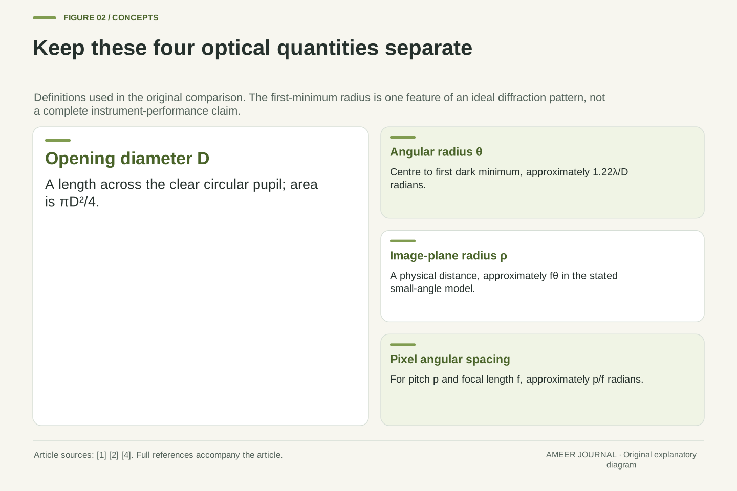
For our comparison, measure from the pattern’s centre to its first dark minimum. Call that angular radius theta. It is not the full diameter across the central region, and it is not a boundary containing all the light: there are rings farther out. The rule is theta approximately equals 1.22 times wavelength divided by opening diameter [1]. The two lengths must use the same unit, and the result is an angle in radians. Stating exactly which part of the pattern we measure prevents a radius from being compared accidentally with a diameter or another width definition.

The ideal point-source response has a central maximum and surrounding diffraction rings. OpenStax derives the circular-aperture first-minimum scale and emphasizes that finite-diameter lenses and mirrors exhibit diffraction even when geometric focusing is ideal [1]. We use θ for the angular distance from the central maximum to the first minimum. This is an angular radius of the central lobe, not its full diameter, not its full width at half maximum and not an encircled-energy boundary enclosing the complete response.

Within the stated small-angle regime, θ≈1.22λ/D in radians. D is large compared with λ in all three designs. The formula identifies one feature of the ideal pattern; it does not supply a complete detector image or a universal definition of recoverable information. A different pupil shape, illumination distribution or obstruction changes the response and requires an appropriate model. The present definition remains useful because it gives every subsequent comparison the same optical reference. In particular, multiplying a radius by two would change the quantity, even if the units still looked correct.

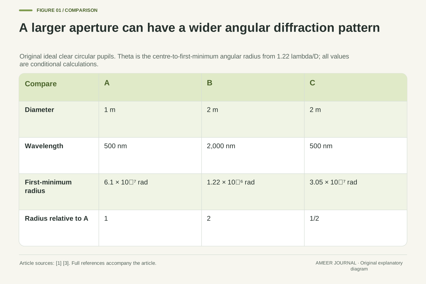
Design A has a one-metre opening and observes a wavelength of 500 nanometres. A nanometre is one billionth of a metre, so 500 nanometres is 0.0000005 metre. Substituting into the rule gives 1.22 × 0.0000005 ÷ 1, or 0.00000061 radian. Design B has a two-metre opening and uses 2,000 nanometres. Its result is 1.22 × 0.000002 ÷ 2, or 0.00000122 radian. B’s opening is wider, yet its first dark minimum lies at twice A’s angular radius because the wavelength increased by the larger factor.

Now introduce C: the same two-metre opening as B, but the 500-nanometre wavelength used by A. Its radius is 0.000000305 radian, half A’s and one-quarter B’s. A versus C shows the benefit of a wider aperture when wavelength stays fixed. B versus C shows the effect of wavelength when diameter stays fixed. Both comparisons use the same circular-opening rule [1]. The examples do not say that a longer wavelength is a poor scientific choice; they show why the purpose of observing it must be considered separately from this angular-width calculation.

Set A=(D=1 m, λ=500 nm), B=(D=2 m, λ=2000 nm) and C=(D=2 m, λ=500 nm). Converting the wavelengths before substitution gives θ_A=6.1×10⁻⁷ rad, θ_B=1.22×10⁻⁶ rad and θ_C=3.05×10⁻⁷ rad. These values follow directly from the rounded-coefficient model, rather than from an instrument specification or a measured point-spread function. Their relative scales are θ_B/θ_A=2, θ_C/θ_A=1/2 and θ_B/θ_C=4. All ratios use the same first-minimum definition, so no radius-to-diameter conversion is hidden.

The general ratio is θ₂/θ₁=(λ₂/λ₁)(D₁/D₂). It exposes the confounding change in A versus B: a fourfold wavelength increase competes with a twofold diameter increase. Comparing A with C isolates aperture, while B with C isolates wavelength. OpenStax supplies the underlying circular-aperture relation [1]; the selected values and comparisons are original. These are spatial angular comparisons at specified wavelengths, not statements about spectral resolving power, source brightness or which wavelength contains the information needed for an astronomical investigation.

Those tiny decimal angles become easier to compare in arcseconds. One degree contains 3,600 arcseconds, while one radian contains 180 divided by pi degrees. Multiplying a radian value by 180 divided by pi and then by 3,600 gives its value in arcseconds. A’s first-minimum radius is about 0.126 arcsecond; B’s is about 0.252; C’s is about 0.0629. An arcsecond is a unit of angle, not a second of elapsed time. Changing the unit makes the numbers more convenient without changing which pattern has the larger radius.

Keep the length conversions equally explicit. The 2,000-nanometre wavelength in B is two micrometres, and 500 nanometres is half a micrometre. They must not be entered as the bare numbers 2 and 500 beside the same diameter unit. OpenStax specifies radians for the diffraction relation [1]. A careful comparison therefore carries both its length units and its angle unit. These angular radii also do not tell us a physical distance between stars: turning a sky angle into a separation requires additional geometry and distance information that our example has not supplied.

Using one radian equal to 180/π degrees and one degree equal to 3600 arcseconds, the conversion factor is 648000/π arcseconds per radian. The three calculated angles are approximately 0.1258215, 0.2516431 and 0.0629108 arcsecond. Reporting them as 0.126, 0.252 and 0.0629 preserves the comparison without suggesting measurement precision. The preceding radian values arise from an already rounded coefficient; the extra decimal digits here are arithmetic outputs, not an uncertainty budget.

Dimensional consistency matters before conversion. For example, 500 nm=5×10⁻⁷ m and 2000 nm=2×10⁻⁶ m. λ/D is dimensionless as a length ratio, with the resulting small angle expressed in radians under the model [1]. An angular quantity can then be converted to another angular unit, but cannot become a physical source separation without a distance assumption. Similarly, a detector-plane distance requires an image-scale parameter. These distinctions explain why an arcsecond specification, a micrometre spot radius and a metre aperture should remain separately labelled in the same comparison.

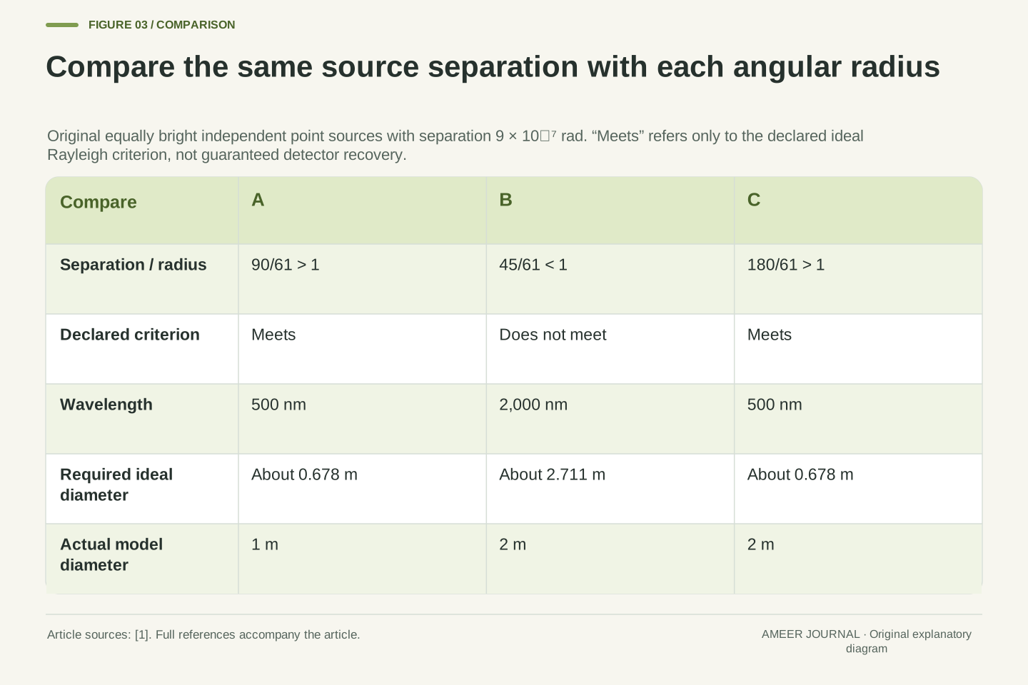
To compare two nearby points, we need a rule as well as a pattern size. The Rayleigh criterion places the centre of one point’s pattern at the first dark minimum of the other when they are just resolved [1]. For this exercise, use two equally bright, independent point sources separated by 0.0000009 radian. We will call the pair within the stated criterion when that separation is at least the first-minimum radius. The relevant comparison uses the centre-to-minimum radius, not the full width across the bright central region.

A’s radius is 0.00000061 radian, smaller than the pair’s separation, so A meets the chosen rule. B’s radius is 0.00000122, larger than the separation, so B does not. C’s radius is 0.000000305, and C also meets it. These results classify our ideal designs under a declared optical criterion. They do not guarantee what a noisy detector will show or prove that every possible inference method must fail below the threshold. We have specified the source pair and the comparison rule, not performed an observation of two actual stars.

The conventional Rayleigh comparison identifies the centre of one ideal point-source pattern with the first minimum of the other at the limiting separation [1]. Adopt it for two equally bright, mutually incoherent point sources, so their intensity responses combine without a fixed interference phase between sources. Let their angular centre separation be δ=9×10⁻⁷ rad. The declared criterion is δ≥θ for the specified pupil and wavelength, with equality representing its conventional boundary.

The exact ratios δ/θ are 90/61 for A, 45/61 for B and 180/61 for C. A and C exceed one; B does not. This establishes the criterion outcomes without claiming a simulated intensity curve or measured dip contrast. Rayleigh is a defined optical comparison, not a universal statistical limit on every estimator or a guarantee of successful detection. Unequal source brightness, noise, optical departures and the inference task would need their own evidence. Our equal-source idealization prevents those unprovided conditions from being silently folded into the three yes-or-no classifications.

The rule can answer a second question: what diameter would just meet our chosen separation at a given wavelength? Multiply 1.22 by the wavelength and divide by the required angle. For the 500-nanometre case, the result is about 0.678 metre. For the 2,000-nanometre case, it is about 2.711 metres. These are conditional boundaries in the same ideal model. A one-metre opening exceeds the first boundary, while B’s two-metre opening falls below the second. That agrees with the classifications we already obtained by calculating the angular radii.

Notice the scaling: keeping the same angular target while increasing wavelength fourfold calls for four times the diameter. Doubling the diameter only offsets a twofold wavelength increase. This is the trade-off behind NASA’s explanation that longer-wavelength observations need a proportionally wider mirror for comparable angular detail [3]. The calculated sizes are not engineering recommendations for an observatory. Real pupils, detectors and scientific requirements need a fuller design. Here the rearranged formula simply lets us check that the forward calculation and the aperture requirement tell a consistent story.

Rearranging δ≥1.22λ/D for positive D and δ gives D≥D_min=1.22λ/δ. At δ=9×10⁻⁷ rad, the two wavelengths yield D_min=61/90 m≈0.677778 m and D_min=122/45 m≈2.711111 m. The ratio of these required diameters is exactly four within the chosen rounded-coefficient model. A and C exceed the first requirement; B does not reach the second. The inequality direction follows because increasing D decreases θ for fixed positive wavelength. At equality the pair is just at the chosen criterion; the inequality does not impose a photon-count condition.

This conditional calculation also clarifies the phrase comparable resolution in a wavelength comparison. Holding θ fixed implies D proportional to λ; holding λ fixed instead gives θ inversely proportional to D. NASA uses the first relationship when explaining why a longer-wavelength observatory needs a wider primary mirror [3]. Neither statement specifies throughput, obscuration, image stability or acceptable signal quality. The derived D_min is therefore a Rayleigh-model boundary for our declared pair, not a complete aperture specification or a promise that a real instrument of that diameter would satisfy every observing requirement.

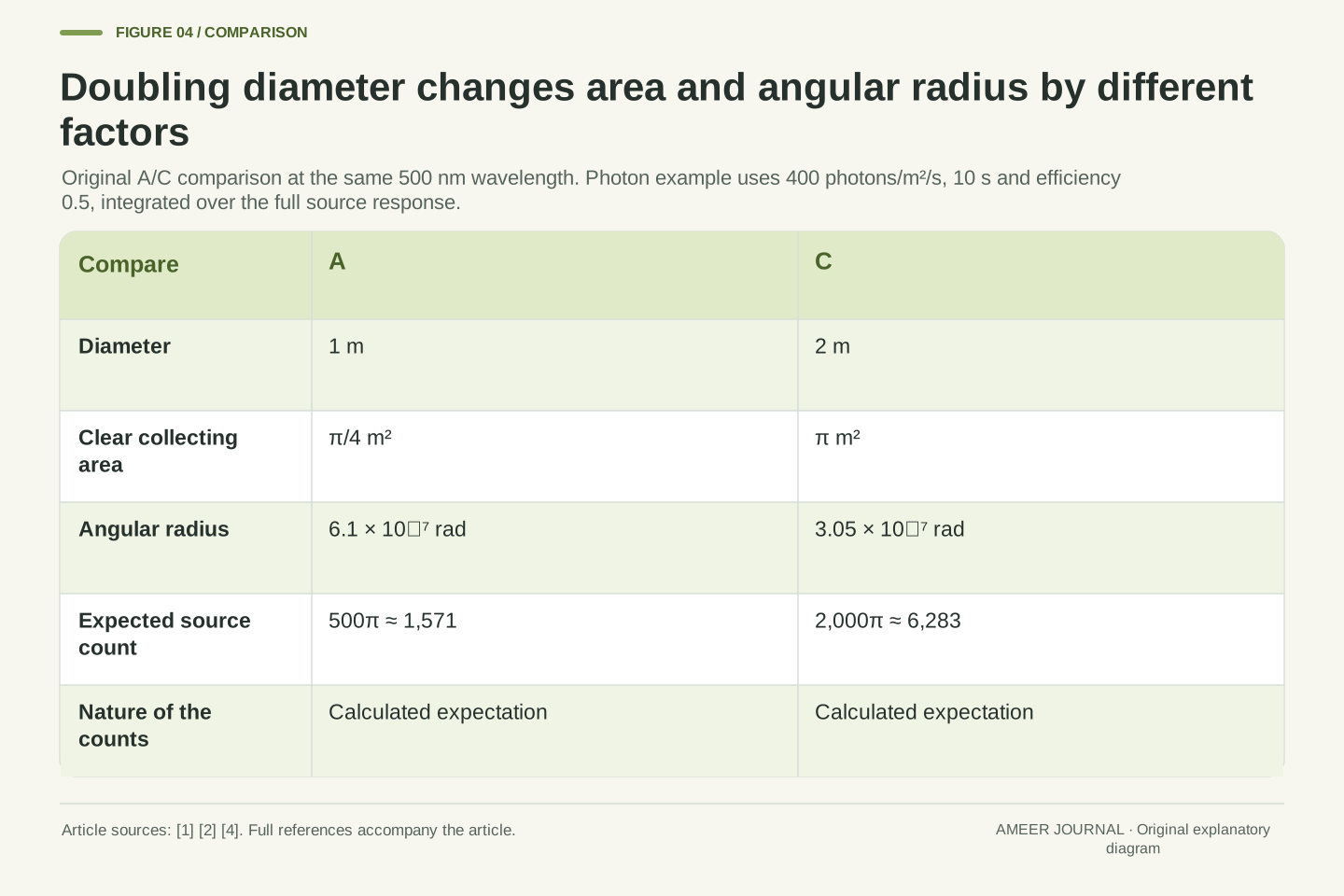
A circular opening’s area is pi times its diameter squared divided by four. A therefore has about 0.785 square metre of clear area, while C has about 3.142 square metres: four times as much. OpenStax distinguishes this light-gathering role from focusing [2]. For an invented matched observation, suppose the same point source supplies 400 photons per square metre each second in the same narrow wavelength band, the exposure lasts ten seconds, and half the collected source photons are recorded. Count the full source response rather than just one central detector pixel.

Those assumptions give expected recorded counts of 500 times pi for A and 2,000 times pi for C: about 1,571 and 6,283. An expected count is an average predicted by the stated rate, so a fractional calculation does not mean a detector records a fraction of an individual photon. C has four times the expected source count and half the angular first-minimum radius of A. The factors differ because area depends on diameter squared. We cannot transfer this photon-count ratio to A versus B without specifying the source’s brightness and instrument efficiency at B’s different wavelength.

For the unobscured circular pupils, collecting area is A_p=πD²/4, giving π/4 m² for A and π m² for C. The area ratio is four, while their angular first-minimum ratio is one-half. OpenStax associates light gathering with aperture area [2], and NASA describes separate wavelength-selection and detection components [4]. To make a count comparison explicit, stipulate identical incident point-source photon flux Φ=400 photons m⁻² s⁻¹ in the same narrow band, exposure t=10 s and aggregate optical/detection efficiency η=0.5.

Integrating the full source response gives expected recorded source counts N=ΦA_p tη: N_A=500π≈1570.796 and N_C=2000π≈6283.185. These are expectation values, not measured integer realizations or a noise model. The fourfold ratio requires the matched spectral flux, duration and efficiency assumptions; it is not a prediction for the longer-wavelength design B. No signal-to-noise ratio, saturation level, background contribution or required exposure is inferred. Likewise, integrated point-source counts do not by themselves specify peak-pixel brightness or the appearance of an extended object.

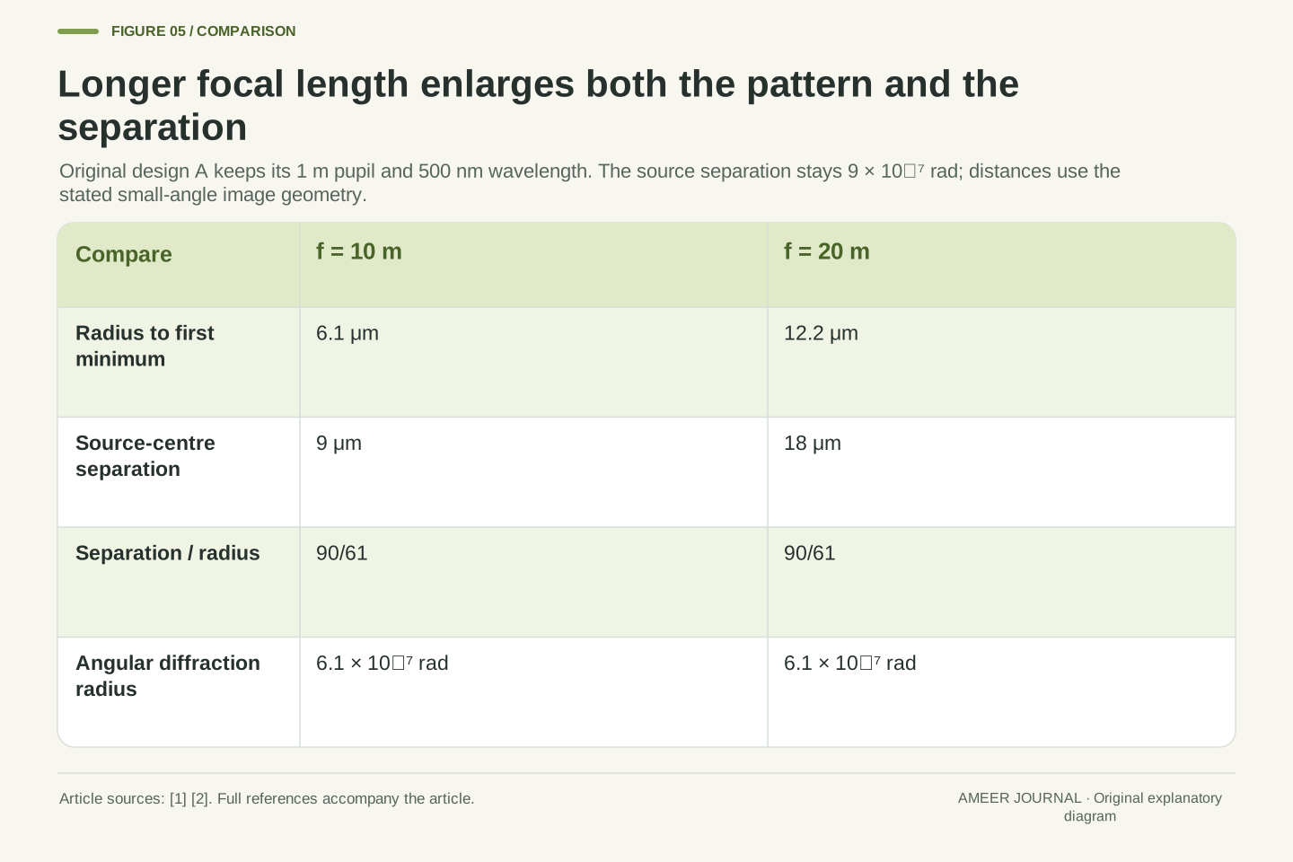
Now keep A’s opening and wavelength fixed, but compare ideal effective focal lengths of ten and twenty metres. Focal length controls the scale of a focused image; it is a different quantity from the opening diameter [2]. In the small-angle geometry here, multiply an angle in radians by focal length to get the corresponding image-plane distance. A’s first-minimum radius becomes 6.1 micrometres at ten metres and 12.2 micrometres at twenty metres. The pattern occupies more physical space on the image plane even though its angle on the sky is unchanged.

Our two point-source centres also move farther apart in that plane. Their 0.0000009-radian separation becomes nine micrometres at the shorter focal length and eighteen at the longer one. Both the centre separation and the diffraction radius doubled, so their ratio stayed the same. Enlarging the image has not changed whether A meets the earlier angular criterion. This is why a large-looking image and fine angular detail are different claims. The example concerns effective optical image scale; it does not imply that the telescope’s physical body must equal either stated focal length.

Under paraxial image geometry, an angular displacement α corresponds to x≈fα, where f is effective focal length. The source explanations of focusing and small-angle geometry provide the basis [1][2]. Hold design A’s D and λ fixed while choosing f=10 m and f=20 m. Its first-minimum focal-plane radius is ρ=fθ_A, giving 6.1 μm and 12.2 μm. No change to θ_A follows merely from this change of image scale. A micrometre is 10⁻⁶ m, which makes the physical-length conversion explicit.

For the same pair, centre separation is d=fδ, giving 9 μm and 18 μm. Thus d/ρ=δ/θ_A=90/61 at both focal lengths. The unchanged ratio is the relevant optical comparison; larger physical dimensions alone cannot demonstrate improved angular discrimination. These equations use ideal near-axis image coordinates, not a measured detector point-spread function or an assertion that physical telescope length equals effective focal length. They also do not require changing the aperture, so the collecting area in this particular comparison remains π/4 m².

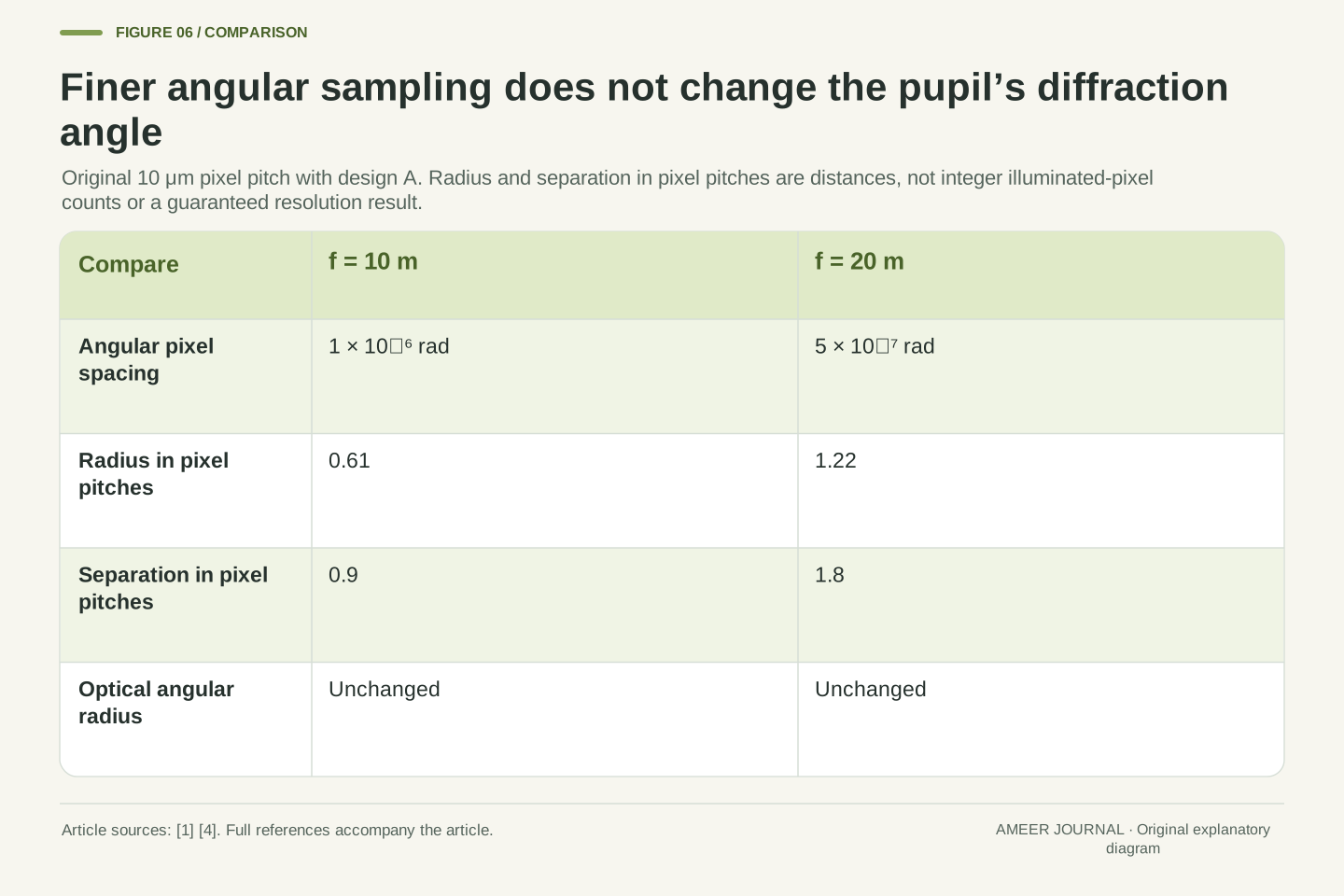
Add an invented detector with pixels spaced ten micrometres apart. At a ten-metre focal length, that pitch corresponds to 0.000001 radian per pixel. At twenty metres it corresponds to 0.0000005 radian per pixel. The longer focal length places the same angular pattern across more pixel spacings. NASA explains that imaging detectors record brightness at positions across the field [4]. That recording grid introduces a separate scale, so a pixel count should not be substituted directly for the opening diameter or the first-dark-ring angle.

In our two image planes, the diffraction radius spans 0.61 and 1.22 pixel spacings, while the source centres are separated by 0.9 and 1.8 pixel spacings. These are simple ratios of distances, not counts of whole illuminated pixels. A pattern can extend across part of a pixel and across several pixels, depending on position. The numbers alone do not guarantee that either detector image reveals two sources. They show why changing image scale can affect how a pattern is sampled while leaving the ideal angular diffraction calculation unchanged.

For a declared pixel pitch p=10 μm, the small-angle sampling interval is approximately p/f. At f=10 m and 20 m, it is respectively 10⁻⁶ and 5×10⁻⁷ rad per pixel spacing. NASA’s instrument description distinguishes detector arrays and their imaging role from the telescope’s optical collection and filtering [4]. Sampling interval, physical pitch and first-minimum optical angle therefore need separate units and definitions even when they appear in one instrument specification.

Dividing the preceding focal-plane distances by p gives ρ/p=0.61 and 1.22 for the radius, and d/p=0.9 and 1.8 for centre separation. These dimensionless values are distances measured in pixel pitches, not integer pixel occupancies. The calculation establishes no sampling-theorem threshold, reconstruction method or guaranteed detection outcome. Pixel response, registration and noise are unspecified. Enlarging the sampled pattern does not alter λ/D, and the same aperture has not acquired additional incident photons merely because its image occupies more detector coordinates.

Observing above Earth’s atmosphere avoids the atmospheric distortion discussed in OpenStax’s space-telescope example, but it does not remove diffraction [1]. A real instrument also has its own optical geometry and image-forming components. NASA describes different mirror arrangements, alignment mechanisms, filters, detectors and observing modes [3][4]. Our clear circular opening deliberately leaves those design details out. Its clean calculation explains a dependence; it should not be pasted onto an actual observatory as if every aperture had the same shape and every image had the same quality.

The word resolution also needs a subject. Spatial resolution concerns separating structure in an image; spectral resolution concerns distinguishing wavelengths in a spectrum. Field of view describes how much sky an instrument covers at once. NASA’s instrument guide separates these ideas and notes that actual resolution depends on instrument and observing mode [4]. A wider field is not automatically finer spatial detail, and our angular first-minimum equation does not calculate spectral resolution. A useful telescope comparison says which quantity matters before treating a single larger number as an overall improvement.

The absence of an atmospheric propagation path does not make a finite telescope pupil diffraction-free. OpenStax explicitly retains diffraction in its space-telescope example and discusses additional optical limitations [1]. NASA’s descriptions of real mirror structures and alignment illustrate why our ideal circular pupil is a model rather than an instrument specification [3]. Obscuration, segmentation, nonuniform illumination, optical aberration and image motion require appropriate response information; the coefficient used here cannot be transferred indiscriminately to every pupil and observing condition.

The instrument guide further distinguishes spatial resolution, spectral resolution and field of view, and qualifies actual resolution by instrument and observing mode [4]. The present θ is an angular spatial measure. It is neither a wavelength-separation metric nor the angular extent of the complete recorded field. Filters also select a band rather than an abstract single wavelength, so a real broadband comparison must identify its spectral conditions. These qualifications leave the original ratio calculations intact while preventing them from becoming unsupported mission-performance or whole-instrument superiority claims.

When a telescope comparison says a larger mirror sees more detail, ask what wavelength is being compared and what detail means. For our ideal designs, A versus C holds wavelength fixed and halves the angular diffraction radius by doubling diameter. A versus B changes both inputs and doubles that radius. If the question is collected light instead, use the area and the matching photon conditions. If it is image size on a detector, use focal length. The sources describe these different optical and instrument roles [1][2][4]; our examples show why the numbers must keep their labels.

A compact explanation can now carry the full result: C’s opening is twice A’s diameter, its clear area is four times larger, and at the same wavelength its first-dark-ring radius is half as large. Under the stated matched observation, its expected source count is four times larger. Enlarging A’s image with a longer focal length changes physical distances and pixel sampling but preserves its angular criterion. Those are useful, checkable conclusions. They leave the actual telescope, observing mode and scientific target to supply the information that a paper aperture comparison cannot provide.

A reproducible comparison records the pupil model, wavelength, chosen optical width or criterion and the units of the result. For a source pair, it also records the separation and source assumptions. The three-design calculation then has an unambiguous interpretation: B/A has λ ratio four and D ratio two, producing θ ratio two; C/A has λ ratio one and D ratio two, producing θ ratio one-half. The Rayleigh classification follows from the same declared δ, rather than from an unlabelled visual impression [1].

Collection and detector questions add their own variables. Expected integrated source counts require spectral photon flux, area, time and efficiency; physical image distances require f; sampling intervals require p/f. The original numbers keep those dependencies explicit without deriving a noise floor or a real observing result. NASA’s mode-dependent instrument description is the practical reminder that an optical relation is only one part of a measurement system [4]. Preserving these distinctions allows a reader to explain why a larger aperture, a larger image and a smaller angular feature can be related without being interchangeable quantities.