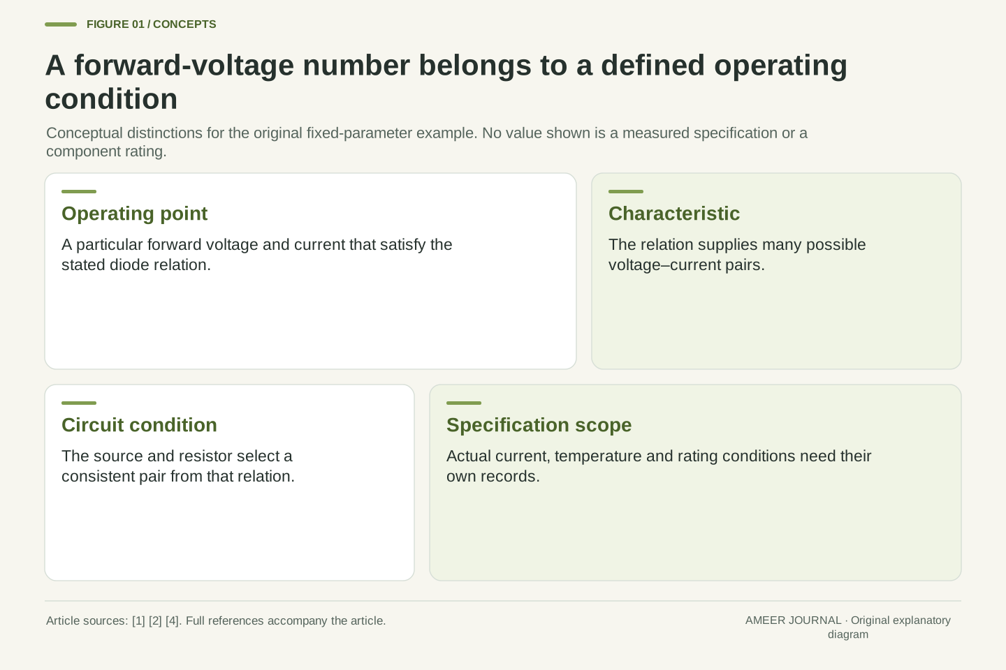
A circuit explanation says that a silicon diode drops about 0.7 volts. Another explanation gives a different forward voltage. Both statements might describe useful approximations, but neither number means much until we know the current and conditions. The forward voltage is a point on a current–voltage relationship. It is not a universal line below which every diode carries exactly no current and above which the current becomes unlimited [1][2].

Analog Devices explains why a constant voltage is often a convenient shortcut: over a chosen range, the voltage can change modestly while the current changes considerably [2]. That convenience should stay attached to its range. We will follow one invented diode curve, then combine it with an ideal resistor and source. The numbers are calculated teaching examples, not measurements of a named component. They let us ask a precise question: does the proposed voltage and current satisfy both the diode’s relationship and the surrounding circuit?

A forward-voltage value describes an operating condition on a diode’s I–V characteristic. Treating 0.7 V as a literal discontinuity confuses a constant-drop approximation with the underlying current relation. OpenStax presents an exponential junction-current model, while Analog Devices describes constant forward voltage as an approximation useful over a selected current range [1][2]. These descriptions are compatible when their roles remain explicit.

This article studies a forward-biased p–n diode through a deliberately assigned smooth DC model. The parameters, current examples, resistor values and source voltages are original assumptions. No device was fitted or measured, and no temperature is inferred from them. We first solve for voltage at specified currents, then solve the coupled resistor–diode operating point. Later comparisons separate error relative to this chosen curve from physical measurement error, and separate local incremental resistance from the ratio V/I. Those distinctions make the familiar voltage shorthand interpretable without claiming that one elementary equation captures every real diode effect.

In a p-type semiconductor, holes are the majority charge carriers; in an n-type region, electrons are the majority carriers. A hole describes a missing electron state that can behave as a moving positive carrier. These labels describe the carrier populations. They are not instructions to imagine one entire block as a positively charged battery terminal and the other as a negatively charged terminal [1][3].

Near the joined regions, carrier diffusion and recombination leave fixed charged impurity ions. The resulting depletion region and electric field oppose further diffusion. At equilibrium, the junction has zero net current even though that internal structure exists [1][3]. Forward bias changes the barrier and makes carrier transfer easier. This is a continuous electrical relationship, not a tiny door that must first click past exactly 0.7 V. The internal built-in potential and the externally measured voltage need their own meanings. Our calculations will describe the terminal voltage under a chosen current condition.

The p and n designations identify majority-carrier types: holes and electrons respectively. Diffusion and recombination near the junction leave ionized acceptors and donors, creating a depletion-region field [1][3]. The bulk-region labels should not be read as a claim that the two entire pieces carry opposite net charges. OpenStax identifies equilibrium with zero net current, while retaining the junction’s internal charge and potential structure [1].

Forward bias reduces the junction barrier relative to equilibrium and changes carrier injection. The built-in potential is therefore not interchangeable with a universal externally applied turn-on threshold. Our subsequent terminal relation is an approximation to current behavior, not a calculation of the spatial electric field, depletion width or every carrier concentration. ROHM’s account supplies the carrier and fixed-ion distinction [3]; its introductory barrier shorthand is not used here as a hard cutoff rule. Keeping the internal structure separate from terminal operating quantities prevents a qualitative junction picture from silently imposing a discontinuity on the mathematical model.

Our imaginary diode uses a smooth relationship: the current grows exponentially as its forward voltage increases. Exponentially means that equal voltage increases can produce approximately equal multiplication factors in current over a suitable part of the curve. The introductory junction equation in OpenStax provides this general shape [1]. We choose the numbers for our example so that its consequences can be inspected.

The current scale is one nanoampere, or one billionth of an ampere, and the voltage scale is 0.050 V. The Technical version writes the complete equation. At zero terminal voltage, this particular formula gives zero net current. For any positive forward voltage it gives a positive current, growing smoothly rather than jumping at a named threshold. These fixed parameters define one teaching curve. They do not claim a particular commercial diode, material recipe or junction temperature. Throughout the calculations, forward voltage means the voltage from the diode’s anode to its cathode, and positive current uses that same forward direction.

Define Vd as anode voltage minus cathode voltage, and I as forward conventional current. Our stipulated relation is I=Is[exp(Vd/s)−1], with Is=1 nA and s=0.050 V. The exponent Vd/s is dimensionless. The physical introductory Shockley form motivates the exponential-minus-one structure [1][3], but the two assigned constants here are explanatory parameters rather than a fit to a component or an assertion of its temperature.

At Vd=0, the exponential equals one and the net current vanishes. For Vd>0, the expression is positive and continuous. The fixed-parameter derivative is dI/dVd=(Is/s)exp(Vd/s), also positive. Thus the curve has no special mathematical discontinuity at 0.7 V. All subsequent operating-point calculations stay in forward DC conditions. We do not extend this simplified expression to predict reverse breakdown, fast transitions or high-current behavior where additional device effects matter. Stating the domain now lets the examples use one consistent relation instead of changing the meaning of a diode between calculations.

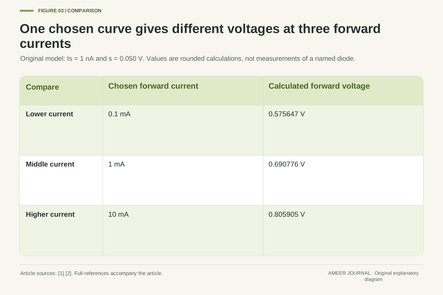
Ask what voltage our model needs for a current of 0.1 milliampere. The answer is approximately 0.575647 V. At 1 milliampere it is about 0.690776 V, and at 10 milliamperes it is about 0.805905 V. A milliampere is one thousandth of an ampere. We have used the same curve for all three answers; nothing about the imaginary diode was changed between them.

The current multiplies by ten at each step while the voltage rises by only about 0.115 V. That helps explain why one rounded voltage can be convenient across some applications, yet incomplete as a general description [2]. The 1 milliampere point happens to sit close to the familiar 0.7 V shortcut. The smaller and larger currents sit elsewhere. If someone supplies only a forward-voltage number, ask which current it belongs to. A second voltage at another current does not automatically show that the first calculation or the component is inconsistent.

Invert the assigned relation for I≥0: Vd=s ln(1+I/Is). Substituting 0.1 mA, 1 mA and 10 mA gives 0.575646773 V, 0.690775578 V and 0.805904788 V respectively. These values are rounded results from the same fixed model. Their spread illustrates why forward current and forward voltage are paired static quantities [4], rather than interchangeable labels for an independently fixed drop.

The two decade increments are approximately 0.115128805 V and 0.115129210 V. They are close, but not mathematically identical: the exact expression retains the added one inside the logarithm. When I is much larger than Is, the decade change approaches s ln 10, approximately 0.115129255 V. This approximation explains the regular spacing without deleting a term across the entire domain. No measured current range is being certified. The result is conditional on the assigned exponential curve, and it locates three distinct operating points rather than three different diode species.

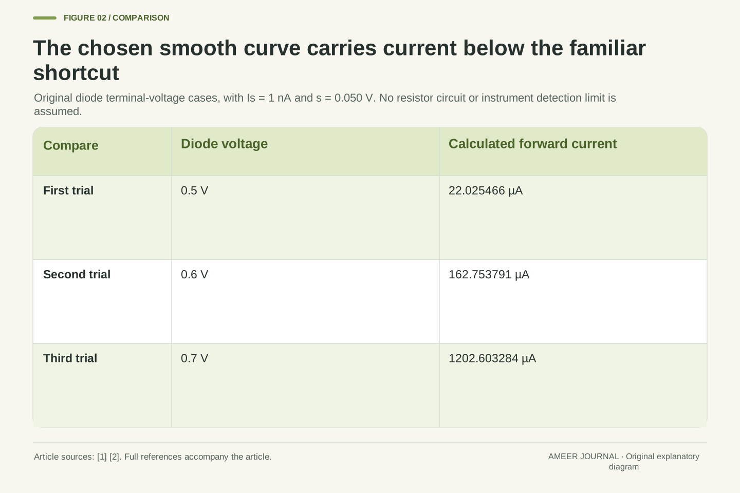
A diagram may make the low-current part look flat. On our curve, 0.5 V gives about 22 microamperes, 0.6 V gives about 163 microamperes, and 0.7 V gives about 1,203 microamperes. A microampere is one millionth of an ampere. Those are very different currents, yet all are positive. Whether the smaller values matter depends on the question the circuit is meant to answer.

Suppose one paper specification calls the diode on when its current reaches 0.1 milliampere. Another uses 1 milliampere. The corresponding voltages are about 0.576 V and 0.691 V in this model. Neither rule changed the curve; each chose a different criterion. Analog Devices discusses a knee and a low-resistance operating region as useful descriptions of a steep characteristic [2]. Such language needs a scale and a purpose. It should not turn a practical boundary into a claim that the current is physically absent at every lower voltage.

The chosen curve gives I(0.5 V)=22.025466 µA, I(0.6 V)=162.753791 µA and I(0.7 V)=1202.603284 µA. These are evaluations at specified diode terminal voltages. They do not yet describe a complete source–resistor circuit. The continuous exponential response can appear to have a knee when displayed on a particular linear scale, but display appearance does not introduce a discontinuity [1][2].

An operational threshold can instead be defined by a current criterion. If on means I≥0.1 mA, its boundary is 0.575646773 V in this model; if on means I≥1 mA, it is 0.690775578 V. Both criteria are well-defined, but neither is an additional material constant. The distinction also prevents an unspecified detection limit from becoming a zero-current claim. Our examples prescribe no instrument resolution or functional load requirement. They show why any binary label derived from a continuous characteristic should identify the condition used to make that label.

Now place the model diode and an ideal 1,000-ohm resistor in one hypothetical series loop with a 1 V ideal source. The same current passes through both elements. The source voltage is shared between the resistor’s drop and the diode’s drop. Analog Devices uses this voltage-budget reasoning when explaining an approximate resistor–diode calculation [2]. Here we will keep the smooth curve and require both relationships to agree.

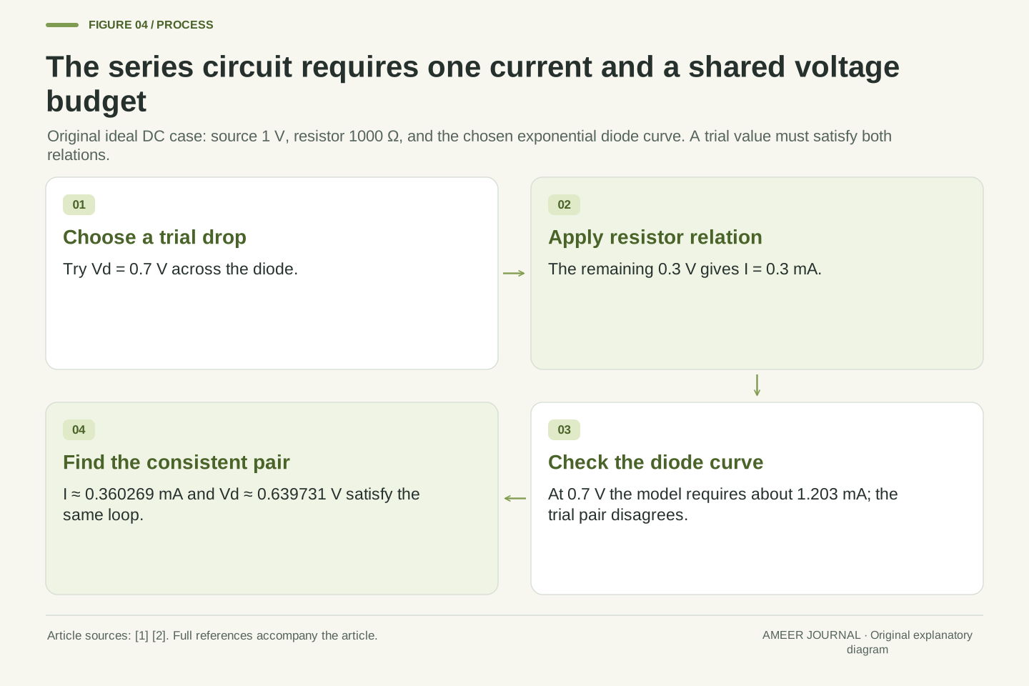
Try assuming that the diode has exactly 0.7 V. That leaves 0.3 V across the resistor, so the resistor relation gives 0.3 milliampere. But our diode curve at 0.7 V requires approximately 1.203 milliamperes. These cannot both be the current in this one series loop. The assumed pair fails the model’s consistency check. Applying the entire 1 V source directly to the diode equation would also ignore the resistor’s drop. We need to find the voltage and current together, rather than assigning each from a different incomplete picture.

For the ideal series circuit, write Vs=Vd+RI with Vs=1 V and R=1000 Ω. The diode and resistor share I. Combining Kirchhoff’s loop relation with the assigned diode equation determines the operating point. The source voltage Vs is not automatically the terminal voltage Vd. The manufacturer’s resistor example likewise allocates part of the source voltage to the forward drop [2].

At the trial value Vd=0.7 V, the resistor relation yields I=(1−0.7)/1000=0.0003 A. The diode relation yields I=0.001202603284 A. Since a single steady series current cannot equal both, that trial voltage is not the intersection of these two characteristics. This is an exact inconsistency within the chosen ideal model, not evidence of a damaged component. It also explains why replacing Vd with Vs in the exponential would solve a different circuit. Both constitutive relations and their shared current must be retained before an operating voltage can be reported.

For the 1 V source and 1,000-ohm resistor, the consistent current is approximately 0.360269 milliampere. The diode has about 0.639731 V, and the resistor has about 0.360269 V. Those two drops add to 1 V. Substituting the diode voltage back into the smooth curve gives the same current. This is the operating point of our declared circuit.

A second case makes the missing hard threshold especially clear. Keep the resistor and curve, but reduce the source to 0.6 V. The solution is still positive: about 54.605 microamperes, with 0.545395 V across the diode and 0.054605 V across the resistor. Even the whole source is below 0.7 V, yet the assigned curve carries current. Whether that amount would perform some real task is a separate question. The calculation establishes agreement between the two model relationships; it does not say that every load would regard this current as useful.

Substitute the inverse diode relation into the loop equation: s ln(1+I/Is)+RI=Vs. For I≥0, its left side has derivative s/(I+Is)+R>0. It starts at zero and exceeds Vs by I=Vs/R when Vs>0. Consequently there is one positive solution within that bracket. The saved arithmetic uses high-precision bisection to locate it; monotonicity supplies the uniqueness argument rather than the numerical search alone.

For Vs=1 V and R=1000 Ω, I≈0.360269482 mA and Vd≈0.639730518 V. The resistor drop RI≈0.360269482 V completes the voltage budget. For the separate Vs=0.6 V case, I≈54.605025 µA, Vd≈0.545394975 V and RI≈0.054605025 V. Displayed values are rounded. The nonzero second solution follows from the assigned continuous model, not a measurement of subthreshold performance. A zero-current branch would belong to a different piecewise approximation and must not be silently substituted into this equation.

Return to the 1 V source and keep the diode parameters unchanged. With a 100-ohm series resistor, the solution is about 2.612 milliamperes and 0.738784 V across the diode. With 1,000 ohms, it is about 0.360 milliampere and 0.639731 V. With 10,000 ohms, it is about 0.0463 milliampere and 0.537132 V. The larger resistance reduces current, and the lower current occupies another point on the same diode curve.

This is why saying the resistor only changes current while the diode always holds exactly 0.7 V describes an approximation rather than this smooth model. The diode’s electrical parameters did not need to change for its terminal voltage to change. The surrounding circuit moved the operating point. The voltage changes are relatively modest compared with the current changes, which is precisely the feature that makes a constant-drop shortcut attractive in some ranges [2]. Whether that shortcut is accurate enough depends on what the final calculation needs to establish.

With Vs fixed at 1 V, the original solutions for R=100 Ω, 1000 Ω and 10000 Ω have currents 2.612156472 mA, 0.360269482 mA and 0.046286828 mA. Their forward voltages are 0.738784353 V, 0.639730518 V and 0.537131716 V. Each pair satisfies both Vd=s ln(1+I/Is) and Vs=Vd+RI using the same Is and s.

The external load relation selects a point from the diode characteristic; it does not modify that characteristic in this fixed-parameter construction. In an actual component, altered current can also change temperature, but that additional effect is excluded here and considered separately below. The present comparison already establishes a changing forward voltage without invoking any parameter drift. Analog Devices’ discussion of steep I–V regions explains the attraction of approximate constant voltage [2]. It does not require us to assert exact constancy when the operating current changes by a large factor.

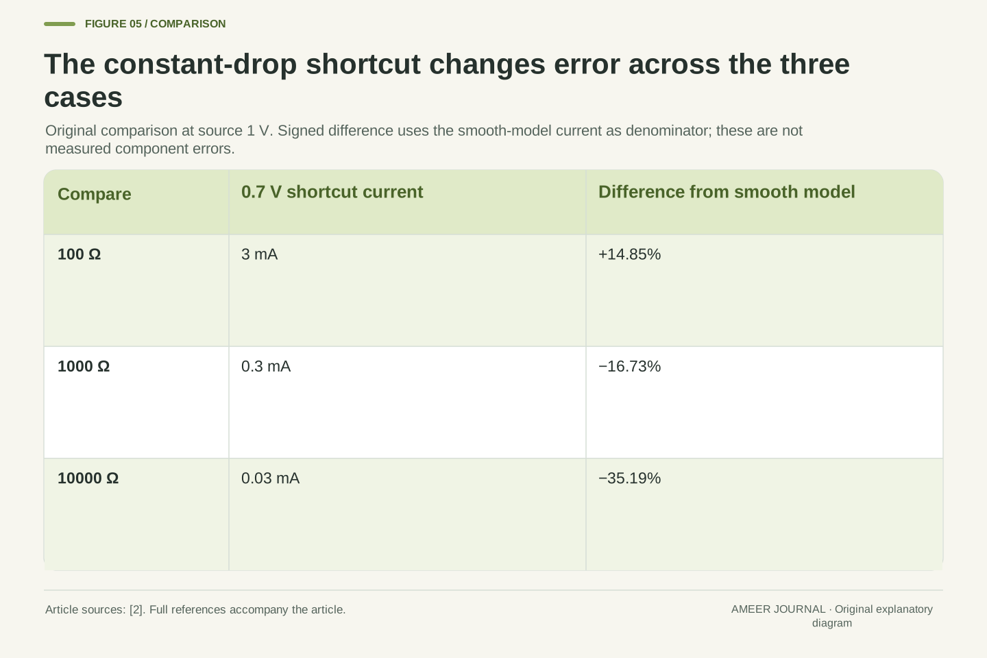
Use a different model now: assign the conducting diode a constant 0.7 V. With the 1 V source and 1,000-ohm resistor, that shortcut predicts 0.3 milliampere. Our smooth model gave approximately 0.360269 milliampere. Relative to the smooth-model current, the shortcut is about 16.73 percent lower. That is a comparison between two declared calculations, not a measured error against a physical diode.

The result changes with the resistor. At 100 ohms the shortcut gives 3 milliamperes, about 14.85 percent above the smooth-model answer. At 10,000 ohms it gives 0.03 milliampere, about 35.19 percent below. Even the direction of the difference changes. A useful approximation therefore needs an intended range and an acceptable difference for the task. The constant-voltage approach described by Analog Devices simplifies analysis [2]; its simplicity does not supply its own accuracy guarantee. Below its chosen threshold, a consistent piecewise model would also need an explicit off rule.

Define the constant-drop approximation as Iapprox=(Vs−0.7 V)/R for the positive-current examples at Vs=1 V. Compare it with Ismooth from the assigned exponential relation using signed relative difference (Iapprox−Ismooth)/Ismooth. For R=100 Ω, 1000 Ω and 10000 Ω, the approximate currents are 3 mA, 0.3 mA and 0.03 mA, with signed differences approximately +14.85%, −16.73% and −35.19% respectively.

The denominator is explicitly the smooth-model current. Neither model is promoted to physical ground truth, and these percentages are not component tolerances. The exercise shows the operating-range dependence of a constant-drop simplification [2]. At a source voltage below 0.7 V, blindly continuing the formula would produce a negative value; a conventional forward-only piecewise approximation instead assigns an off branch. That is a separate model choice. Its zero current should not be presented as the result of the positive smooth solution already calculated for Vs=0.6 V.

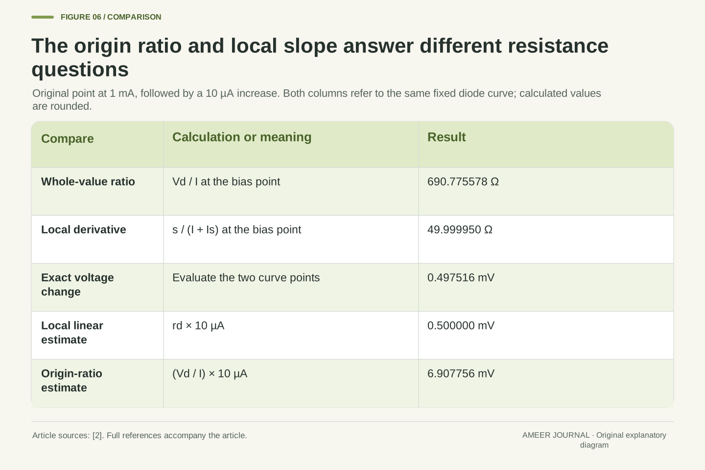
At the model’s 1 milliampere point, the diode voltage is about 0.690776 V. Dividing the whole voltage by the whole current gives about 690.8 ohms. That ratio draws a line from the graph’s origin to this point. It does not tell us how steeply the curve changes right beside the point.

Analog Devices defines incremental resistance using the local slope of the current–voltage curve [2]. Our model gives about 50 ohms there. Increase the current by only 10 microamperes, from 1.000 to 1.010 milliamperes. The exact voltage change is approximately 0.497516 millivolt. The local 50-ohm estimate gives approximately 0.500000 millivolt, which is close for this small change. A millivolt is one thousandth of a volt. Using the 690.8-ohm whole-value ratio would instead predict about 6.91 millivolts. The two resistance numbers answer different questions, even though they refer to the same starting point.

At I=1 mA, the origin ratio is Vd/I≈690.775578 Ω. Differentiate the inverse relation to obtain incremental resistance rd=dVd/dI=s/(I+Is)≈49.999950 Ω. This is the reciprocal local I–V slope described by Analog Devices [2]. A nonlinear device can have both quantities without contradiction; they use a secant from the origin and a tangent at the bias point respectively.

For ΔI=10 µA, the exact increment is s ln[(Is+I+ΔI)/(Is+I)]≈0.497516 mV. Linearization gives rdΔI≈0.4999995 mV. Substituting the origin ratio instead gives (Vd/I)ΔI≈6.907756 mV, which is not the local derivative estimate. The close tangent result is specific to a sufficiently small change around this point; it does not turn the diode into a 50 Ω resistor over its whole characteristic. Frequency-dependent impedance is another matter because this static derivative includes no junction capacitance or transient charge behavior.

Our examples held the current scale and voltage scale fixed. Real diode characteristics depend on the device and its conditions. Analog Devices discusses temperature and self-heating, while ROHM explains that reverse saturation current changes with temperature [2][3]. It would be incomplete to alter just one number in our equation and announce a real temperature prediction while silently freezing everything else.

The steady curve also cannot tell us how quickly a diode responds when voltage reverses. ROHM lists reverse recovery and capacitance separately from forward current and voltage [4]. Nor does a calculated point establish that a component can safely operate there. Maximum ratings, temperature conditions and any stated duration are separate specification questions [4]. These limits help interpret the result rather than erase it: the original arithmetic correctly solves its chosen DC model, while a real device comparison needs the relevant characteristic, operating conditions and rating information in addition to a convenient voltage shorthand.

Fixed Is and s are assumptions of the original calculation. They do not imply that a real junction retains both parameters as its temperature changes. Analog Devices discusses thermal dependence and self-heating [2], and ROHM explicitly notes temperature dependence of reverse saturation current [3]. Changing only the exponential voltage scale while treating the current scale as constant would therefore be a restricted parameter exercise, not an established physical temperature coefficient.

The model also omits high-current series effects, reverse breakdown and transient charge or capacitance. ROHM distinguishes static current/voltage characteristics from recovery and capacitance, and distinguishes electrical characteristics from maximum ratings and temperature conditions [4]. No switching-time or allowable-dissipation result follows from our solved DC point. A real specification must supply the applicable conditions and whether a quoted value is typical, bounded or a rating. The article’s numbers remain internally meaningful within their declared relation; additional physical questions require additional evidence rather than extra decimal places in the same equation.

Here are two complete statements about our example. At a prescribed current of 1 milliampere, the chosen diode curve gives about 0.690776 V. In the separate circuit with a 1 V ideal source and a 1,000-ohm resistor, the same curve settles at about 0.360269 milliampere and 0.639731 V. The statements describe different operating points and agree with one another.

When reading a forward-voltage claim, keep that relationship visible. Look for the associated current, the relevant conditions, and what kind of number is being reported. A typical curve point, a guaranteed limit and a rough calculation are different records [2][4]. If a resistor is present in the explanation, check that its voltage drop and the diode’s drop share the available source voltage consistently. The familiar 0.7 V value can still be a useful shorthand. Its usefulness comes from the approximation and range being understood, rather than from a sudden universal switch hidden inside the junction.

A complete statement identifies the independent conditions and the resulting pair. For the prescribed-current problem, I=1 mA implies Vd≈0.690775578 V. For the coupled circuit problem, Vs=1 V and R=1000 Ω imply I≈0.360269482 mA and Vd≈0.639730518 V. The diode parameters are identical in both. Neither the source voltage nor a remembered nominal drop can replace the solved terminal condition.

Preserve the distinction between a characteristic point, an approximation and a specification limit when reporting the answer [2][4]. The original examples show three separate checks: invert the diode relation at the requested current, solve the complete voltage budget when the current is unknown, and evaluate any simplification against an explicitly chosen reference and tolerance. They also distinguish whole-value and incremental ratios. Those checks explain why different forward voltages can all be consistent, and why an isolated 0.7 V label cannot determine a circuit’s current or establish every condition of its operation.