What you’ll take away
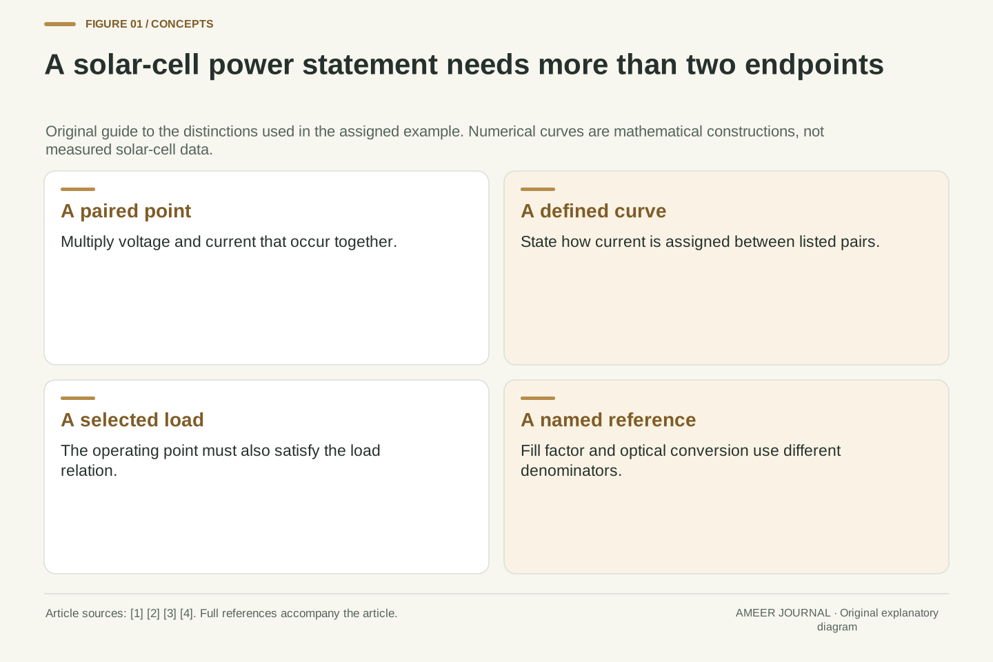
- Open-circuit voltage and short-circuit current occur at different points; their product is not delivered endpoint power.
- The largest listed product and the maximum of a defined continuous curve answer different questions.
- Two continuous decreasing constructions can share the same sparse pairs while having different maxima.
- A load selects an operating point; knowing a curve’s maximum does not guarantee operation there.
- Fill factor, optical conversion efficiency and energy require different reference information.
Two impressive endpoint numbers do not occur together
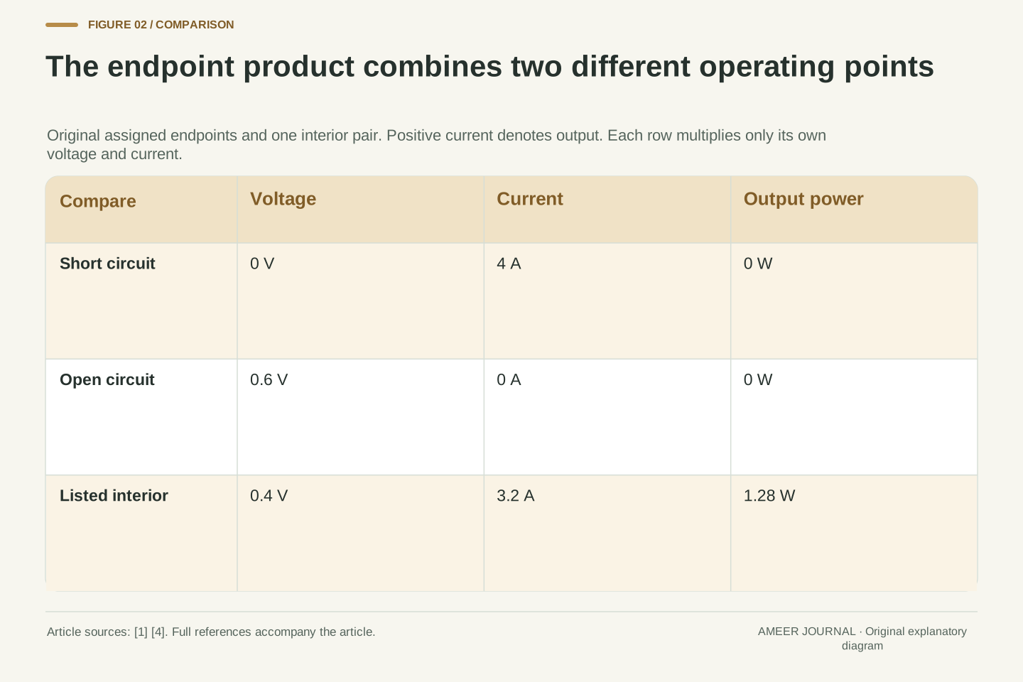
A solar-cell record gives an open-circuit voltage of 0.6 volts and a short-circuit current of 4 amperes. Multiplying them gives 2.4 watts. That arithmetic is correct, but it has combined values from two different operating points. At open circuit, the current is zero. At short circuit, the terminal voltage is zero. Neither endpoint therefore delivers 2.4 watts of electrical output; each has voltage times current equal to zero [1][4].
The useful question is which voltage and current occur together between those endpoints. We will answer it using an original five-point example and two explicitly invented curves. The example is mathematical, with no solar cell measured or electrical equipment operated. It shows why the endpoint product is a reference quantity, why the largest listed power need not be the curve’s maximum, and why even a known maximum does not force an attached load to use it. Keeping those questions separate turns a short specification into something we can interpret.
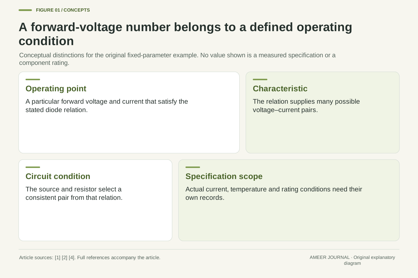
Electrical output power at a specified DC operating point is P=VI. The short-circuit current Isc is evaluated at V=0, while the open-circuit voltage Voc is evaluated at I=0 [1][4]. Their product VocIsc therefore combines coordinates from different points on the characteristic. It is not the power at either endpoint and does not, by itself, identify the maximum-power point.
The original fixture assigns Voc=0.6 V and Isc=4 A, making the endpoint product 2.4 W. Five paired values will constrain two continuous, decreasing mathematical constructions. Neither is claimed as measured data, a fitted physical cell model or output from photovoltaic software. We distinguish a maximum over a finite list, a maximum over a completely defined interpolation, an operating point imposed by an ideal load, and ratios using different denominators. These distinctions concern the information in a record, rather than the installation or operation of real solar equipment.
Keep the current convention and the conditions attached
Current–voltage diagrams can use different sign conventions. A diode drawing may count current into the device as positive, while a solar-cell output drawing counts generated current leaving it as positive. PVEducation explains this change of presentation when discussing an illuminated cell [1]. In our example, positive current means output supplied to the load, and positive voltage times positive current means delivered electrical power. All the listed points use that convention.
The points also belong to one stipulated set of conditions. A real photovoltaic characteristic depends on conditions such as irradiance and cell temperature; Sandia’s modeling guide includes both among the influences represented in a cell model [3]. We do not take a voltage from one lighting condition and a current from another. Such a combination would no longer describe the endpoint rectangle of one curve. A useful record keeps the pair, its conditions and its sign convention together, even when a summary displays only a few headline numbers.
Adopt the generating-quadrant convention V≥0 and I≥0, with I positive out of the cell into an external load. Then VI is positive delivered power. This convention differs from a passive-sign diode plot in which generated current may appear negative; the sign change does not represent a different device [1]. The article’s domain is the assigned branch 0≤V≤0.6 V, and all products refer to that branch.
A characteristic must also be tied to a common condition set. Sandia’s single-diode description treats the I–V curve as continuous and identifies parameters influenced by temperature and irradiance [3]. Our later piecewise-linear construction is deliberately a different, elementary definition; it is not an evaluation of that physical model. The source establishes why conditions belong with a curve, not the truth of our invented point values. Combining Voc and Isc from separate conditions, or silently changing current orientation between columns, would invalidate an otherwise correct multiplication before any maximization is attempted.
Start with five complete voltage–current pairs
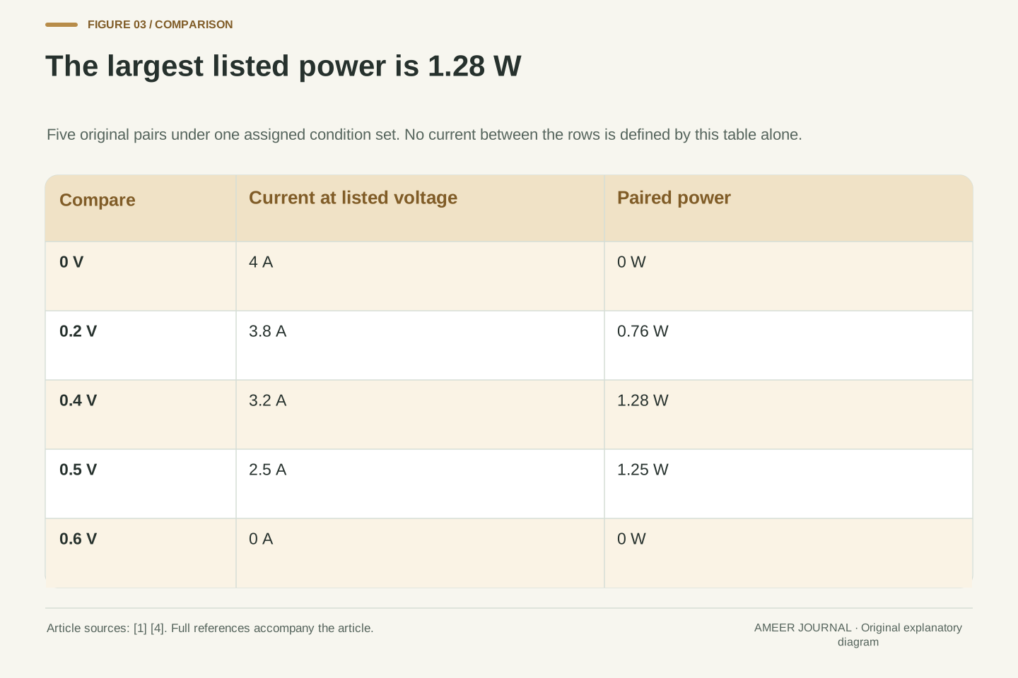
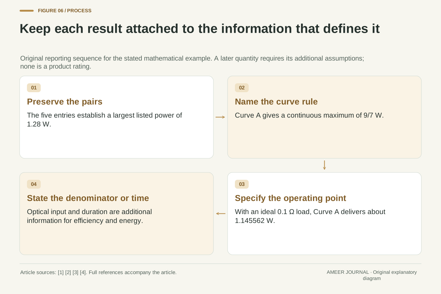
Here is the whole original list, with voltage first and current second: (0 V, 4 A), (0.2 V, 3.8 A), (0.4 V, 3.2 A), (0.5 V, 2.5 A), and (0.6 V, 0 A). Multiply within each pair. The five powers are 0 W, 0.76 W, 1.28 W, 1.25 W and 0 W. The middle pair supplies the largest power among these five entries, even though it has neither the largest voltage nor the largest current.
This pairing rule is the essential part of the calculation. At 0.5 V, the assigned current has fallen to 2.5 A, so power is slightly smaller than at 0.4 V with 3.2 A. Increasing one factor does not guarantee an increase in their product when the other factor changes. Photovoltaic measurement guidance accordingly describes obtaining corresponding current and voltage values across a characteristic [4]. Our list is invented, but each multiplication respects the same requirement: the two factors must identify one operating point.
Define the finite set S={(0,4),(1/5,19/5),(2/5,16/5),(1/2,5/2),(3/5,0)}, where each first coordinate is in volts and each second coordinate in amperes. The associated powers are exactly 0,19/25,32/25,5/4,0 watts. Thus max over S of VI is 32/25 W at (2/5 V,16/5 A), or 1.28 W at (0.4 V,3.2 A). Moving to the next listed pair raises voltage by 0.1 V but lowers power by exactly 0.03 W. The paired current decrease determines why selecting a larger voltage alone does not maximize their product.
The record consists of five paired operating points, not independent lists from which the largest V and largest I may be selected. The current decreases as voltage rises across these entries, but their product first increases and then decreases. Source guidance on I–V characterization treats paired acquisition and appropriate conditions as part of determining the characteristic [4]. Here the values are assigned exactly, so rounding and measurement uncertainty are absent from the fixture. They would become separate questions for actual observations; their absence in this calculation is an assumption, not a statement about real instrumentation.
The best listed point is a claim about the list
We can already make one complete statement: 1.28 W is the largest power in our five-point list. We cannot yet say that no unlisted voltage produces more. The gap between 0.4 V and 0.5 V contains many possible voltages. A table with five rows does not specify every current between its rows, even if a chart draws a neat connecting line without explaining what that line means.
This distinction matters when two reports appear to disagree. One may report the largest recorded product, while the other estimates a peak between recorded points. The second report has added a method or model, and that addition needs to be visible. Photovoltaic characterization guidance discusses sufficient point density and ways of locating maximum power [4]. It does not make every sparse list a complete continuous curve. In our example, the next step is to state an interpolation rule openly, so the stronger claim follows from a defined mathematical object.
A finite maximization and a continuous maximization have different domains. The exact value max over S of VI=32/25 W says nothing by itself about the products at points outside S. In particular, monotonic decrease of the listed current values does not determine how current decreases between adjacent entries. A plotted segment may be a graphical guide or a defining interpolation; these roles should not be conflated.
Actual characterization methods address sampling, interpolation or fitting when estimating maximum power [4]. This article does not execute one of those measurement procedures. Instead, it first preserves the finite-set result, then adds an explicit piecewise-linear definition. The resulting continuous maximum is exact for that definition, while its relation to a real cell would require additional evidence. Keeping the domain in the wording prevents extra decimal places or a smooth display from turning an unobserved interior value into an actual measurement. It also makes two results comparable without assuming that they answered the same question.
Define every connecting segment before using the curve
Call our first construction Curve A. Join each neighboring pair with a straight line and use that line to assign the current at every voltage between them. This is a rule, rather than a claim that real solar cells have four straight portions. For example, halfway from 0.4 V to 0.5 V is 0.45 V. Halfway from 3.2 A to 2.5 A is 2.85 A, so Curve A assigns 2.85 A at 0.45 V.
The four segments fit at their shared endpoints, and current falls continuously from 4 A to zero. Those features make the construction easy to inspect. They also let us calculate power at any point in the stated interval. At 0.45 V, power is 1.2825 W, already above the largest value in the original table. The difference is small, but its existence answers the logical question: the best listed point and the maximum of a defined continuous curve need not be identical. We still have to find the actual peak of Curve A.
To keep numerical coefficients dimensionless, write v=V/(1 V) and i=I/(1 A). Define Curve A by i=4−v for 0≤v≤0.2; i=4.4−3v for 0.2≤v≤0.4; i=6−7v for 0.4≤v≤0.5; and i=15−25v for 0.5≤v≤0.6. Adjacent formulas agree at their shared endpoints. Each has negative slope, and the complete branch is continuous and nonnegative. Recover units after calculating: vi is the numerical power in watts because (1 V)(1 A)=1 W. The third segment’s physical current–voltage slope is −7 A/V; the dimensionless form keeps those units separate from its numerical coefficient.
These are the straight-line interpolants of the five assigned pairs. They are not a simplification derived from Sandia’s single-diode parameters [3]. The power in watts has numerical value vi. At v=0.45, the third segment gives i=2.85 and P=1.2825 W, exceeding 1.28 W. This interior comparison already disproves equality between the finite maximum and Curve A’s maximum. It does not locate the global maximum, because another interior point could be higher. A complete maximization must inspect each segment and the places where the defining formula changes.
Check the interior and the boundaries for maximum power
On Curve A, the highest power occurs at a voltage of 3/7 V, approximately 0.428571 V, with a current of exactly 3 A. Their product is 9/7 W, approximately 1.285714 W. The Technical version checks each straight segment and all their meeting points. The result is a maximum of the defined curve, so it is a stronger statement than selecting the largest of five products.
The curve’s peak exceeds the table’s best value by exactly 1/175 W, about 0.005714 W. Relative to the curve’s maximum, that difference is 1/225, or about 0.4444 percent. Naming the denominator matters: we are expressing the gap as a share of the model maximum, not as a share of the tabulated value. A small gap may be acceptable for some purpose, but no required tolerance was supplied here. The useful conclusion is that the two answers have different definitions, and our explicit model makes their difference calculable.
For any segment i=a−bv, the numerical power is av−bv². Its stationary point is v=a/(2b), provided that point lies inside the segment. Curve A gives formal candidates 2,11/15,3/7 and 3/10. Only 3/7 belongs to its own segment, 0.4≤v≤0.5. The others must not be evaluated as if their local formulas applied over the entire voltage range.
Compare the valid stationary point with every knot. At v=3/7, i=6−7(3/7)=3, giving P=9/7 W; this exceeds all five endpoint-of-segment products. Consequently it is the global maximum on the defined branch. The gap from the finite maximum is 9/7−32/25=1/175 W. Dividing that gap by 9/7 W gives 1/225, about 0.4444 percent. PVEducation describes maximum power through the stationary condition for a differentiable I–V relation [2]; here the piecewise construction additionally requires boundary checks, since a maximum could occur where adjacent segment derivatives differ.
The same five entries can conceal a different peak
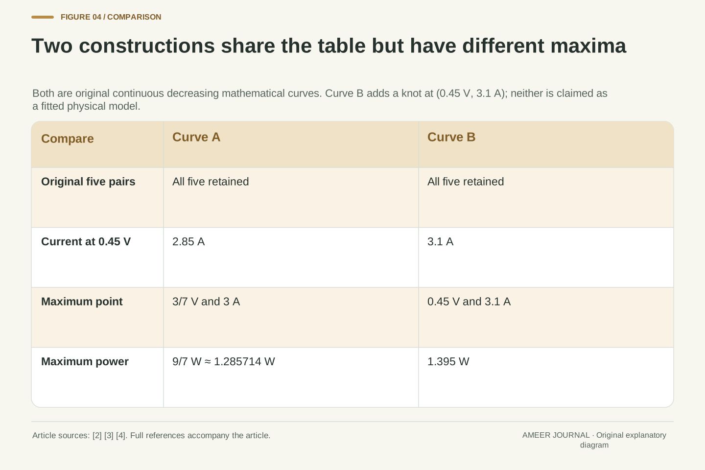
Now construct Curve B. Keep all five original pairs, but add one new point between 0.4 V and 0.5 V: at 0.45 V, assign 3.1 A. Join neighboring points with straight lines again. Current still falls continuously as voltage rises. Every entry in the original five-row table remains unchanged, yet the new point has power 0.45×3.1=1.395 W. Checking the segments shows that this point is Curve B’s maximum.
Curve A gives only 2.85 A at the same 0.45 V. The sparse table cannot choose between those two interior values because it contains neither. This is a deliberately mathematical counterexample under the stated continuity and decreasing-current conditions. It does not establish that either curve is a physically fitted solar cell. A real cell model would impose additional constraints. The example establishes the narrower conclusion we need: the original five values, even with a generally falling current, do not uniquely determine the continuous maximum.
Define Curve B by adding the knot (v,i)=(9/20,31/10). Replace Curve A’s third segment with i=4−2v on 0.4≤v≤0.45 and i=17/2−12v on 0.45≤v≤0.5. Leave the other three segments unchanged. Both new pieces meet at i=3.1 and retain the original endpoint values 3.2 and 2.5. Thus every original observation is shared, while continuity and strictly decreasing current are preserved. At the unlisted voltage 0.45 V, the constructions differ by 0.25 A and 0.1125 W. A comparison restricted to the original five rows cannot reveal either difference.
The formal power vertices of the new pieces are v=1 and v=17/48, both outside their respective intervals. Power therefore reaches its maximum at the intervening knot, where P=(9/20)(31/10) W=279/200 W=1.395 W; all other knots are lower. This maximum is not Curve A’s 9/7 W. The constructions prove non-uniqueness within the declared mathematical class, not physical realizability under a single-diode parameterization. Additional physical assumptions could reduce that class, but they would be additional information rather than consequences of the five pairs alone.
A load selects an operating point on the chosen curve
Return to Curve A and connect an ideal resistor in the mathematical example. A resistor requires its voltage and current to satisfy voltage equals current times resistance. The operating point must satisfy that rule and Curve A at the same time. With resistance 0.1 ohm, the consistent point is about 0.338462 V and 3.384615 A, producing about 1.145562 W. Knowing the curve’s higher maximum has not made this load operate there.
A resistance of exactly 1/7 ohm does select the maximum point: 3/7 V and 3 A. Increasing resistance to 0.2 ohm selects 0.5 V and 2.5 A, giving 1.25 W. The middle resistance is best only for this assigned curve and this simple load family. It is not a universal resistance for solar cells. These examples explain the distinction between power available at a curve’s maximum and power delivered at the operating point. They do not describe a controller that automatically finds or follows that maximum.
For an ideal positive resistance R, the load relation is I=V/R. Intersect it with Curve A rather than assigning the maximum-power voltage independently. For R=1/10 Ω, the solution lies on the second segment: V=22/65 V, I=44/13 A and P=968/845 W≈1.145562 W. In dimensionless coordinates this load gives i=10v, so the second segment requires 4.4−3v=10v. The resulting v=22/65 lies in that segment’s permitted interval. The increasing load-current line and decreasing cell-current curve have a unique intersection on the specified branch.
At R=1/7 Ω, the intersection is V=3/7 V and I=3 A, exactly the maximum-power point. This resistance is Vmp/Imp for the fixed construction, not a universal characteristic or an incremental-resistance value. At R=1/5 Ω, the solution is V=1/2 V, I=5/2 A and P=5/4 W. That point belongs to two neighboring segment boundaries but is one operating point, so it must be deduplicated when solving segment by segment. No control dynamics, tracking algorithm or physical load test is implied by these static intersections.
Fill factor compares maximum power with the endpoint product
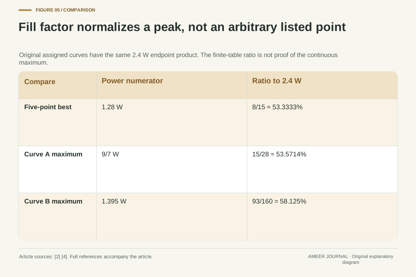
The endpoint product does have a useful role. Fill factor divides the maximum electrical power by open-circuit voltage times short-circuit current [2][4]. For Curve A, divide 9/7 W by 2.4 W. The result is 15/28, about 0.535714, or 53.5714 percent. Both the numerator and denominator refer to the same assigned curve and conditions. The ratio describes how much of that endpoint-product reference is reached at the maximum-power point.
For Curve B, the endpoints are unchanged but the maximum is 1.395 W, so fill factor becomes 0.58125, or 58.125 percent. The different result reflects a different interior shape. If we divide only the largest tabulated power, 1.28 W, by 2.4 W, we get about 53.3333 percent. That is a ratio based on the finite table, not proof of the continuous fill factor without a method for finding the peak. None of these percentages yet tells us how much incoming light became electrical power.
Use the definition FF=Pmp/(VocIsc) [2][4]. For Curve A, FF=(9/7)/(12/5)=15/28≈0.535714. For Curve B, FF=(279/200)/(12/5)=93/160=0.58125. Their common endpoint rectangle does not force a common fill factor because Pmp depends on the interior characteristic. The normalization cancels power units, making FF dimensionless.
The finite table instead gives (32/25)/(12/5)=8/15≈0.533333 for its largest listed product. Describing that number as a measured or estimated fill factor requires the appropriate acquisition and peak-estimation context; our five assigned entries alone establish only the finite ratio. Under our nonnegative decreasing constructions, every product lies below VocIsc, but the definition does not say that the unattainable combination (Voc,Isc) is an operating point. It also does not compare electrical output with incident radiant power. That second ratio needs an optical input quantity which neither endpoint supplies.
Light-conversion efficiency needs a different denominator
To calculate a light-to-electricity ratio, add two more assigned facts: a relevant illuminated area of 0.01 square metre and irradiance of 1,000 watts per square metre. Together they give 10 watts of incident radiant power. These are extra assumptions, not values recovered from the voltage–current table. Photovoltaic characterization guidance defines conversion efficiency using electrical output divided by incident irradiance times the stated area [4].
Using Curve A’s maximum electrical output, the ratio is (9/7 W)/(10 W), or about 12.8571 percent. This can coexist with a fill factor of about 53.5714 percent because the denominators are different. At the 0.1-ohm operating point, the electrical-to-incident-power ratio is instead about 11.4556 percent. The optical input was held fixed; the load used a different point on the electrical curve. These numbers belong to our assigned example. They are not ratings for a real product, nor evidence that one technology converts light better than another.
Assign illuminated reference area A=0.01 m² and irradiance G=1000 W/m² over that area. Incident power is AG=10 W. The conversion-efficiency denominator is therefore optical input power, whereas the fill-factor denominator is VocIsc [4]. The area definition and irradiance conditions must accompany a real efficiency result; they cannot be inferred from electrical endpoints alone.
At Curve A’s maximum, η=Pmp/(AG)=(9/7)/10=9/70≈0.128571. At its R=0.1 Ω load point, P/(AG)=(968/845)/10=484/4225≈0.114556. The latter is the delivered-to-incident-power ratio at that selected operating point, rather than the maximum conversion efficiency of the assigned curve. FF=15/28 remains unchanged because the curve and its endpoint reference remain unchanged. Distinguishing these quantities prevents a change in electrical loading from being mislabeled as a change in fill factor, or a fill-factor percentage from being reported as a percentage of sunlight converted.
A maximum-power point does not determine energy over time
The calculations so far describe one fixed set of conditions. If those conditions change, the relevant current–voltage relationship can change too [3]. A resistance that selected the maximum of Curve A is not thereby guaranteed to select the maximum of a different curve. A specification at one condition therefore cannot tell us, by itself, the energy supplied throughout a day or the behavior of a system that adjusts its operating point.
For a separate time example, suppose that output power really remains at 9/7 W for half an hour. Then energy is 9/14 watt-hour, about 0.642857 Wh. The constant power and duration are stated assumptions. They do not follow from a momentary maximum-power label. When power varies, its contributions across time must be accumulated. This separates another pair of questions: a characteristic can identify possible power at particular conditions, while an energy result also needs the conditions, operating choices and durations over the period being described.
The curve, its maximum and the selected load intersection are conditional quantities. Temperature and irradiance dependence in photovoltaic modeling means that changing the conditions requires a corresponding characteristic, rather than automatic reuse of the same Vmp, Imp or preferred resistance [3]. Our construction fixes those conditions and contains no temporal evolution or controller policy.
Energy requires an integral of actual output power over time. In a separately stipulated constant-power interval, P=9/7 W for Δt=1/2 h gives E=PΔt=9/14 Wh. This result uses the maintained-power assumption explicitly; it is not a daily yield or an inference about tracking performance. If a time sequence instead uses different curves or load points, each power belongs to its own interval before integration. The distinction is useful even without a weather forecast: a maximum-power value supplies neither elapsed time nor evidence that the system stayed at that maximum throughout the interval.
Report the data, the added rule and the quantity actually found
Imagine receiving two summaries of our original table. The first says that the highest listed output is 1.28 W. The second says that the maximum is about 1.285714 W. Before deciding which is wrong, ask what the second summary used between the rows. With Curve A’s straight-line rule, both statements are correct. With Curve B’s additional point, the continuous maximum is instead 1.395 W. A clear report makes the added information visible rather than presenting all three numbers as competing measurements.
For a useful record, keep the paired values and their common conditions, identify any interpolation or physical model, and name whether the result is a finite-list maximum, a continuous maximum or a load operating point. If a percentage is reported, preserve its denominator and the point supplying its numerator. If energy is reported, include the time assumptions. Those details let another reader reproduce the calculation and see exactly where new evidence would matter. Two endpoint numbers remain useful, but they cannot silently supply the missing shape, load choice or optical input.
A reproducible numerical report should distinguish its evidence from its completion rule. Here S supplies five assigned pairs; Curve A supplies a particular interpolation; the stationary-and-boundary search supplies Pmp=9/7 W; and an ideal load relation supplies a separate operating point. Curve B demonstrates that the original S alone does not determine the same Pmp. These are dependencies of the calculation, not interchangeable labels for a single observation.
Retain the condition set, sign convention, paired values, interpolation or physical-model assumptions, maximum-search domain and any load constraint. For FF retain the matched VocIsc reference; for conversion efficiency retain the area and irradiance; for energy retain the power history or its explicit simplifying assumptions. The resulting record allows independent recomputation and an informed comparison with another report. It also locates uncertainty honestly: changing an interior model is different from correcting a paired value, while changing a denominator changes the reported quantity even when electrical power stays the same.
Sources & further reading
Explore the references behind this guide. External pages may change after our review.
- IV Curve | PVEducationPVEducation · Accessed 7 Nov 2026
- Fill Factor | PVEducationPVEducation · Accessed 7 Nov 2026
- Single Diode Equivalent Circuit Models – PV Performance Modeling Collaborative (PVPMC)Sandia National Laboratories / PVPMC · Accessed 7 Nov 2026
- Current-voltage characteristics - PVMETPVMET / Michael Rauer, Fraunhofer ISE · Accessed 7 Nov 2026
Article updated 7 Nov 2026.
Found something we should revisit?
Good explanations get better with thoughtful feedback.