What you’ll take away
- A navigation fix is a computed estimate, not a direct observation of a device on a map.
- Timing becomes an apparent range; clocks, propagation and geometry must still be handled.
- Four measurements explain a basic four-unknown problem, but count alone does not prove a reliable solution.
- Tightly grouped repeated fixes can still share an offset from an independent reference.
- Separate position error from an incorrect destination or other map-data problem.
A location dot is a calculated answer
Your map shows a neat dot beside a building. It is easy to treat that dot as a direct observation of where you are, rather like seeing yourself in a photograph. Satellite navigation works differently. A receiver processes radio signals and calculates a position from measurements. ESA describes the receiver's output as a solution for position, velocity and time. [5] A solution can be available even when some of its inputs are imperfect.
That distinction explains an everyday puzzle: the app has found you, yet it puts you on the wrong side of the street. Obtaining a fix and demonstrating the accuracy needed for a particular task are separate achievements. GPS.gov distinguishes the quality of signals transmitted in space from the accuracy experienced by a receiver, which also depends on its surroundings, geometry and design. [3]
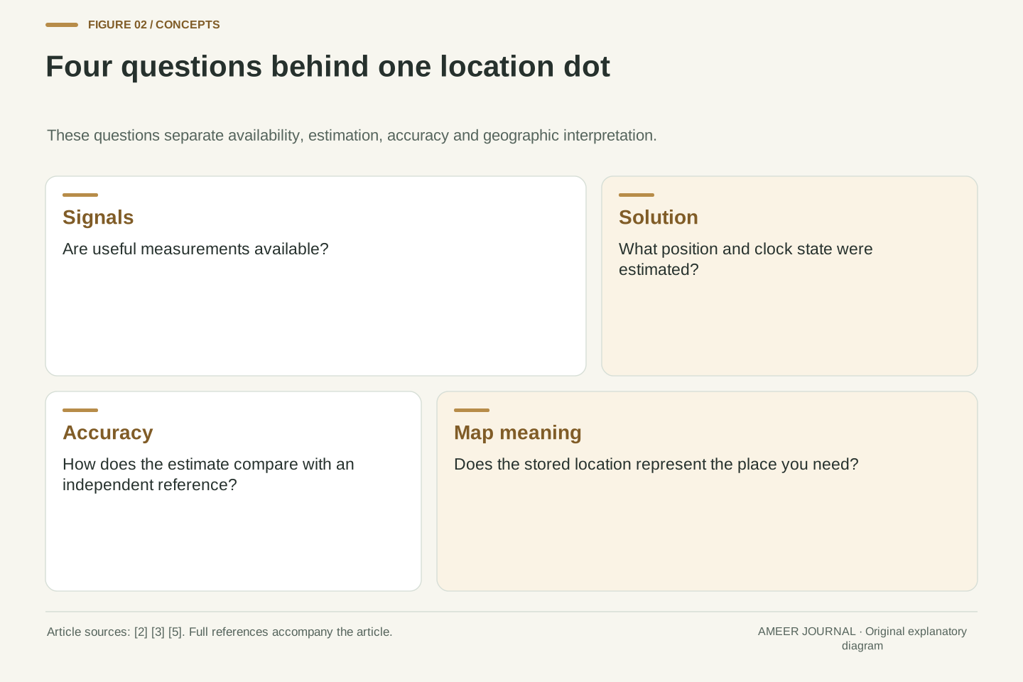
We will follow the measurement through to the dot, using deliberately invented examples. No phone or navigation receiver was tested for this article. The aim is to separate four questions: did the receiver obtain usable signals, what position did it calculate, how close is that estimate to reality, and does the map describe the intended place correctly? Answering one does not automatically answer the other three.
A navigation fix is an estimated state produced from observations and a model. ESA's receiver introduction describes position, velocity and time as computed outputs obtained by processing satellite signals. [5] The presence of coordinates therefore establishes that an estimation process returned a result; it does not establish the uncertainty, external accuracy or application suitability of that result. Those require additional evidence and a declared evaluation criterion.
Keep the measurement layer distinct from the display layer. Signal-in-space accuracy is not identical to user positioning accuracy, as GPS.gov explicitly explains. Geometry, signal blockage, propagation conditions and receiver characteristics contribute to the latter. [3] A mapping application adds another interpretation: the coordinates must be related to streets, entrances or other stored geographic features. An apparently wrong destination can involve either layer.
The following examples are transparent calculations rather than performance tests. They isolate propagation-time scale, receiver clock bias and the difference between repeatability and accuracy. They do not model a complete operational GNSS receiver, establish a product ranking or specify an uncertainty radius for a phone. Keeping those boundaries explicit makes the mechanism useful without turning a simplified explanation into an unsupported navigation guarantee.
The receiver listens for a known pattern
GPS includes satellites, ground infrastructure and receivers. NASA's introductory account explains that the receiver listens to satellite signals and uses measurements from several satellites to work out its location. [1] This is a receiving task: the measurement is not a satellite photograph of your device or a direct report of which shop you are standing outside.
One useful part of the signal is a recognizable ranging code. The receiver compares an incoming code with a locally generated version and shifts the local version in time to find a match. ESA calls this correlation. The resulting timing relationship helps form an apparent distance. [2] Think of recognizing the same pattern at two different positions on a timeline, rather than measuring an angle with a protractor.
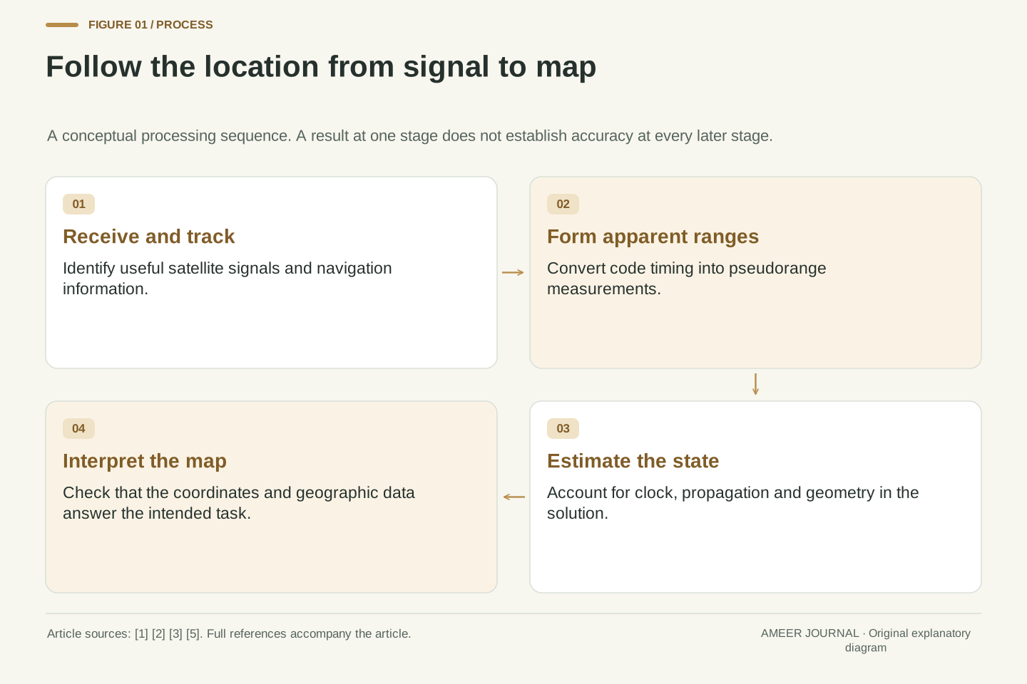
That pattern match is one stage, not the final location. The receiver must also use navigation information and account for clock and propagation effects. ESA describes acquisition, tracking, measurements and the navigation solution as related steps. [5] If a device reports that it can see a satellite, ask whether the signal is actually being used in a valid solution; a list of detected signals is not itself a position-quality report.
The basic architecture separates transmitted signals, supporting ground infrastructure and the user receiver. NASA's overview identifies those three components and describes the receiver as listening for satellite signals. [1] The navigation mechanism considered here is receive-side ranging and state estimation. It does not depend on a satellite imaging the receiver, and this description says nothing about separate application-level communication or data sharing.
For a code observable, the receiver correlates the received ranging code with a local replica and adjusts their relative timing. ESA's basic-observables reference relates that code delay to an apparent propagation interval, multiplied by the vacuum speed of light to form a pseudorange. [2] Code alignment should not be confused with an independent measurement of a geometric bearing or with a complete solution for the receiver coordinates.
Acquisition and tracking maintain useful signal relationships, while navigation data and modeled corrections contribute to the later position solution. ESA's receiver introduction distinguishes these processing functions. [5] Accordingly, satellite detection, tracked signals, accepted measurements and a solved state are different diagnostic quantities. A meaningful receiver comparison states which quantity is being reported rather than treating a larger number of visible signal entries as proof of a more accurate position.
A tiny timing difference becomes a large range term
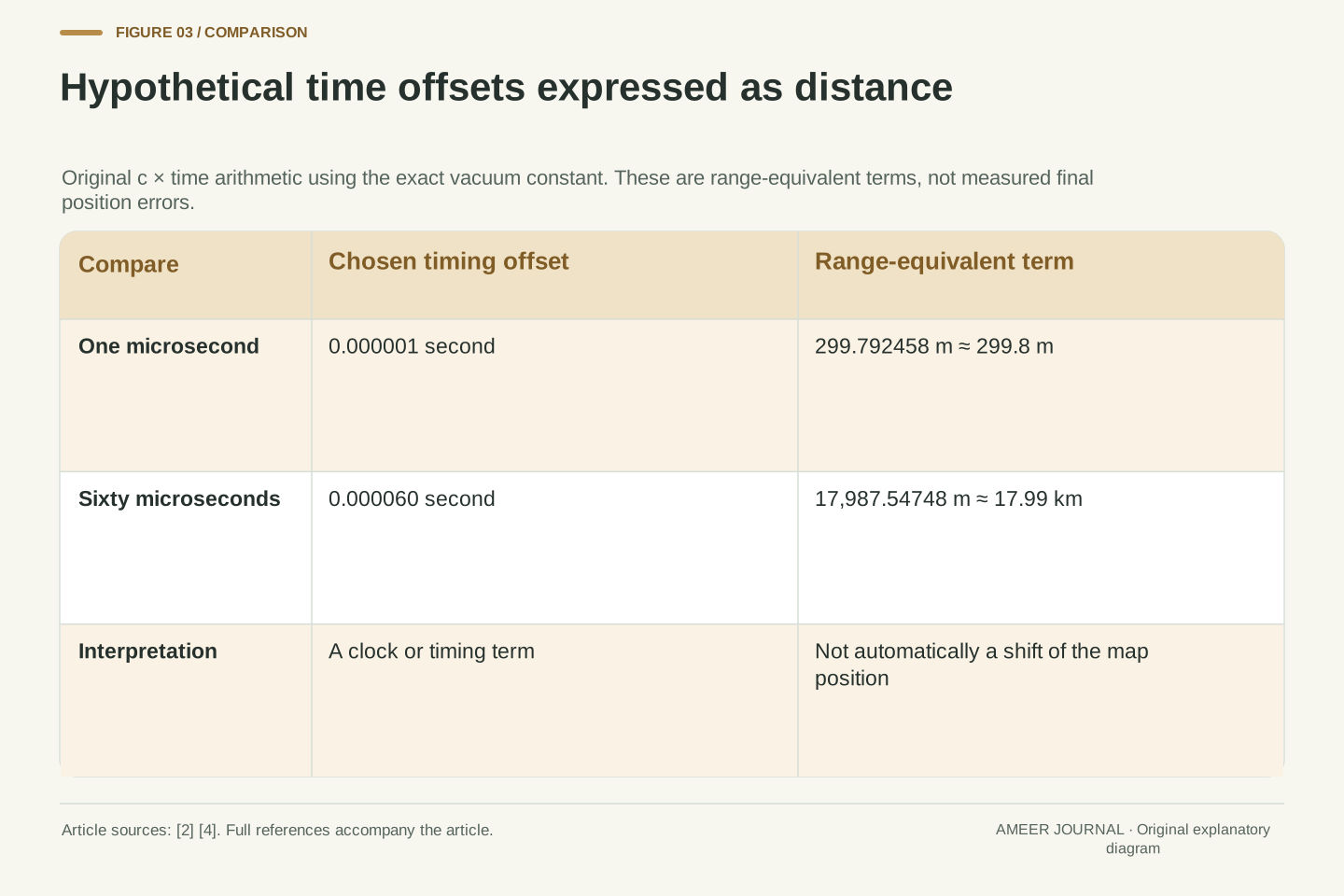
Light in a vacuum travels at exactly 299,792,458 metres per second, the value listed by NIST. [4] That number also sets the conversion scale used when navigation timing is expressed as distance. In an ideal calculation, a timing difference of one microsecond—one millionth of a second—corresponds to about 299.8 metres. This is a unit conversion, not a measured error from a device.
For another invented value, sixty microseconds corresponds to about 17.99 kilometres. Such examples explain why timing deserves careful treatment. They do not mean that a phone whose clock is sixty microseconds off must display a location 17.99 kilometres away. A receiver clock offset is something the navigation calculation can estimate, alongside position, rather than an error that must be blindly converted into a shift on the map.
Also keep the vacuum calculation separate from the real signal path. ESA's measurement description includes atmospheric delays, clock differences and other contributions in the apparent range. [2] The multiplication by the speed of light establishes the scale; it does not remove those contributions. A long-looking distance discrepancy may belong to the timing model rather than representing an equally large error in the final coordinates.
Use c = 299,792,458 m/s, the exact vacuum constant documented by NIST. [4] An illustrative time offset delta-t = 1 microsecond produces the range-equivalent term c delta-t = 299.792458 m. For delta-t = 60 microseconds, the term is 17,987.54748 m, or about 17.99 km. Both are original dimensional calculations on chosen offsets, not observations of a receiver's clock or final positioning error.
A common receiver clock offset appears in multiple simultaneous pseudoranges and can be estimated as a shared parameter. Therefore, c times that offset is not automatically the displacement of the position estimate. Position and clock are separated through the multi-observation solution under its modeling and geometry assumptions. A residual error that the model fails to account for has a different interpretation from a clock parameter that the model successfully estimates.
The vacuum speed belongs in the observable definition, while actual propagation effects require additional terms or corrections. ESA explicitly lists ionospheric and tropospheric contributions, instrumental effects, multipath and noise. [2] Treating c delta-t as a perfectly corrected geometric distance would erase the very distinction the term pseudorange is intended to preserve. The calculation illustrates sensitivity to time, not an assertion of vacuum propagation through the real atmosphere.
Why position and the receiver clock are solved together
In an ordinary three-dimensional problem, location needs three coordinates. If the receiver's clock also differs from the navigation time reference, that adds another unknown. Several distance-like measurements are needed to separate those unknowns. NASA's simplified account uses four or more satellites to explain a position fix. [1] The number is a starting point for understanding the problem, not a promise that any four detected signals are sufficient in every situation.
Imagine trying to choose both your place on a map and the correction for a clock that affects every measured distance. Changing the position changes different distances in different ways. Changing the common clock offset shifts the timing-based distances together. With suitable independent information, the calculation can distinguish those patterns. This is why a receiver does not have to carry a perfectly synchronized clock before it can begin solving the problem.
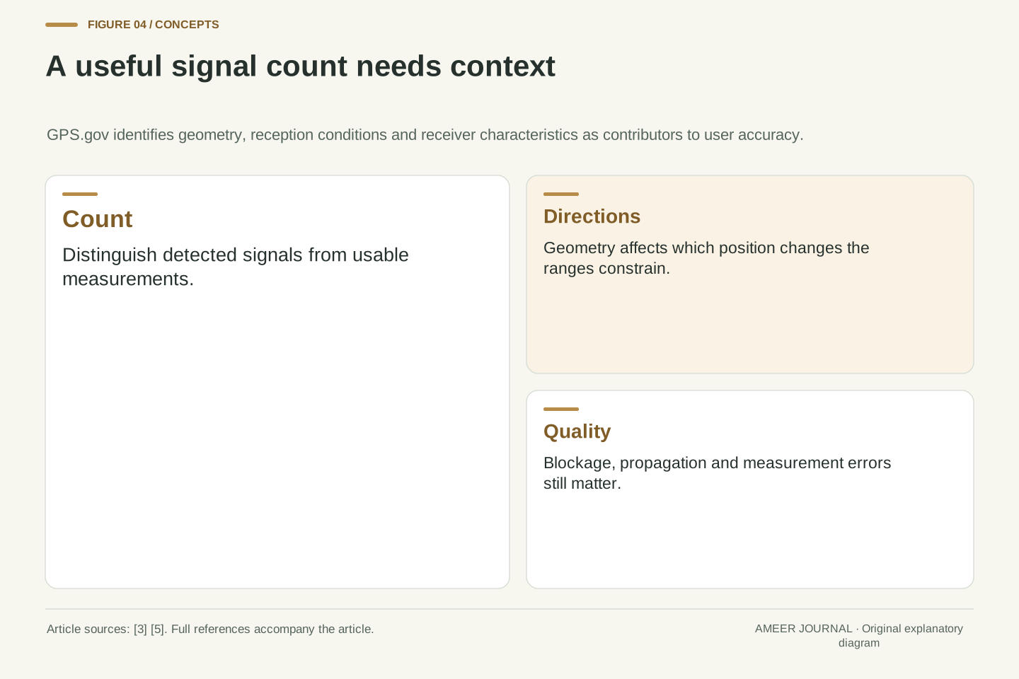
The simple count assumes a suitable set of measurements and one shared receiver-clock unknown. Additional constraints or a more complex receiver model can change the calculation. Even with enough measurements on paper, poor directions or corrupted signals can make the result unreliable. The useful question is whether the observations support the required solution, not whether an icon has reached a magic number.
In a simplified single-time-reference code solution, the unknown state contains x, y, z and a receiver clock offset b. After suitable satellite corrections, write each modeled observation schematically as p_i = distance(x, s_i) + cb + d_i + e_i. Here s_i is the relevant satellite position, d_i collects modeled propagation or other corrections, and e_i represents remaining measurement/model error. This is a simplified expression of the pseudorange terms described by ESA. [2]
Four independent scalar observations are the basic count for four unknowns; NASA's four-or-more-satellite explanation communicates that ordinary positioning principle. [1] An adequate local solution also requires informative geometry and a suitable model. Counting observations does not demonstrate matrix rank, reliable measurements or external accuracy. Additional satellites can supply redundancy, but an unexamined extra observation is not automatically beneficial evidence.
The statement is deliberately limited to this model. Known-height constraints, extra system-time offsets, dynamic states or other measurements can change the unknowns and estimation structure. No universal receiver algorithm is inferred from the four-parameter sketch. Its purpose is to show why a common clock offset and a geometric coordinate change have different signatures across multiple ranges, allowing them to be estimated together rather than conflated.
Pseudorange is an honest name for an unfinished measurement
The word pseudorange can sound as if the receiver has made up a distance. It means something more useful: the measured quantity resembles a distance but still includes effects besides the direct geometric separation. ESA explains that the transmit and receive times belong to different clocks, and that the observable also includes propagation and instrument effects. [2] Naming it carefully tells you what still needs to be modeled.
For example, the atmosphere affects the signal, and reflected paths can complicate reception near structures. GPS.gov identifies obstruction and environmental conditions as contributors to poorer positioning. [3] Correcting a known contribution can improve the model, but it does not prove that every remaining effect has disappeared. A receiver can be doing real calculations with real signals while still producing an imperfect position.
When reading a technical claim, ask which layer improved. Was a timing measurement cleaner? Was a clock or propagation term modeled better? Did the final coordinates become closer to an independent reference? Those are related achievements, but they are not the same claim. A smaller intermediate error needs a demonstrated connection to the result that matters to your task.
A code pseudorange contains geometric separation plus timing and propagation terms, rather than serving as a direct tape-measure observation. ESA identifies receiver and satellite clock offsets, atmospheric contributions, instrumental delays, multipath and receiver noise in its observable model. [2] The geometric term itself concerns the satellite at emission and receiver at reception, so a complete implementation needs a consistent time and coordinate treatment.
Our compact equation groups effects for explanation; it is not a replacement for an operational measurement model. A known or estimated correction reduces a specified contribution. Residual error can still reflect omitted behavior, parameter error or measurement noise. GPS.gov's separation between signal-in-space quality and user accuracy reinforces why a favorable satellite specification cannot be transferred directly to the local coordinate solution. [3]
Evaluate improvement at its stated boundary. A ranging statistic, a state-estimation residual and an externally measured position discrepancy describe different quantities. Internal agreement can be useful without establishing truth. For a performance claim, require a clearly defined reference, operating conditions, metric and evaluation interval. Do not substitute the number of decimal places in a coordinate for an independent uncertainty assessment, or interpret a corrected observable as proof of an error-free position.
Directions matter as well as the number of signals
Several measurements can tell you nearly the same thing if they come from very similar directions. Imagine asking several people to estimate how far you are from points clustered on one side of a large room. Their answers may constrain movement toward that side better than movement across it. This is an analogy about information, not a numerical model of satellite positions.
The same broad issue is why GPS.gov includes satellite geometry among the factors affecting accuracy. [3] Range uncertainty and position uncertainty are connected through the layout of the observations. You cannot determine the second by reading only one distance-error number. The arrangement can also help explain why two sessions with similar signal counts need not provide equally useful location estimates.
Do not turn that observation into a simple rule that more satellites always fix every problem. Signal quality, obstruction and the receiver's handling of the measurements still matter. The defensible conclusion is narrower: count, quality and geometry belong together. When a technical comparison omits the observing conditions, you do not have enough information to assign its result to a different street or device.
The range-to-position mapping depends on the directional geometry of the observations. In a linearized solution, different satellite directions provide different sensitivities to changes in the receiver coordinates. Closely aligned directions can leave some state combinations less well constrained than others. GPS.gov explicitly includes satellite geometry when distinguishing user accuracy from range-error performance. [3] No numeric dilution-of-precision value is assigned here without an actual geometry.
This explains why a scalar range error cannot simply be copied into a universal horizontal-position error. The estimation model, measurement weighting and geometric configuration determine how observation errors influence coordinates and clock. Our room analogy illustrates the information imbalance; it does not reproduce a GNSS covariance calculation or establish an error bound for a real acquisition.
Additional usable observations can improve redundancy and geometry, but the quality and treatment of those observations remain important. Avoid ranking receivers only by a visible-satellite count or comparing accuracy figures from unspecified environments. A meaningful report keeps the acquisition configuration, usable observations, obstruction context and reference method attached to its metric. Otherwise, differences caused by the environment can be mistaken for an inherent product advantage.
A tightly grouped dot can still be in the wrong place
Suppose a known reference point is at coordinates (0, 0) on a small local grid, measured in metres. Four invented fixes are (8, 2), (9, 1), (8, 1) and (9, 2). These points sit close together. Their average is (8.5, 1.5), and each lies about 0.71 metres from that average. The receiver would look reassuringly steady in this made-up example.
Yet the average is about 8.63 metres from the known reference. The small spread did not prove small error. We calculated those distances with ordinary plane geometry; they are not measurements of GPS performance. The example separates repeatability—how closely repeated answers group—from accuracy relative to an independently known location.
Waiting for more tightly clustered points cannot, by itself, prove that a shared offset has gone away. Nor does one accurate-looking point establish that later points will behave the same way. If your question is whether a position meets a required tolerance, define the reference and the error measure. A smooth map animation supplies a different kind of evidence from a comparison against known coordinates.
Use an explicitly hypothetical local Cartesian reference at (0, 0) m and four estimated positions: (8, 2), (9, 1), (8, 1) and (9, 2) m. Their arithmetic mean is (8.5, 1.5) m. Each estimate differs from the mean by 0.5 m in each axis, so its radial distance from the mean is sqrt(0.5² + 0.5²) = 0.7071 m. This is the constructed sample's radial spread, not a confidence interval.
The mean's distance from truth is sqrt(8.5² + 1.5²) = sqrt(74.5) = 8.6313 m. The tight cluster therefore coexists with a substantial bias in this toy dataset. No particular GNSS error mechanism is assigned to that bias; the numbers illustrate the logical distinction between internal repeatability and external accuracy rather than diagnosing a receiver.
Averaging can only support the conclusions warranted by the error assumptions and reference information. Repeated observations need not be independent, and a common offset need not vanish. Report the metric actually computed—sample scatter, mean error, individual error distribution or another defined statistic. Do not label the 0.71 m sample radius as 95% accuracy, and do not infer a probability guarantee from four intentionally chosen coordinates.
A correct coordinate can still meet a wrong map
The receiver and the map can fail in different ways. GPS.gov notes that mapping software can mislead users even when GPS hardware is functioning. [3] An address may be represented by a point that is not the entrance you need, or the displayed route may rely on different geographic information from the position estimate. Check the actual destination information before concluding that the satellite measurement must be the only problem.
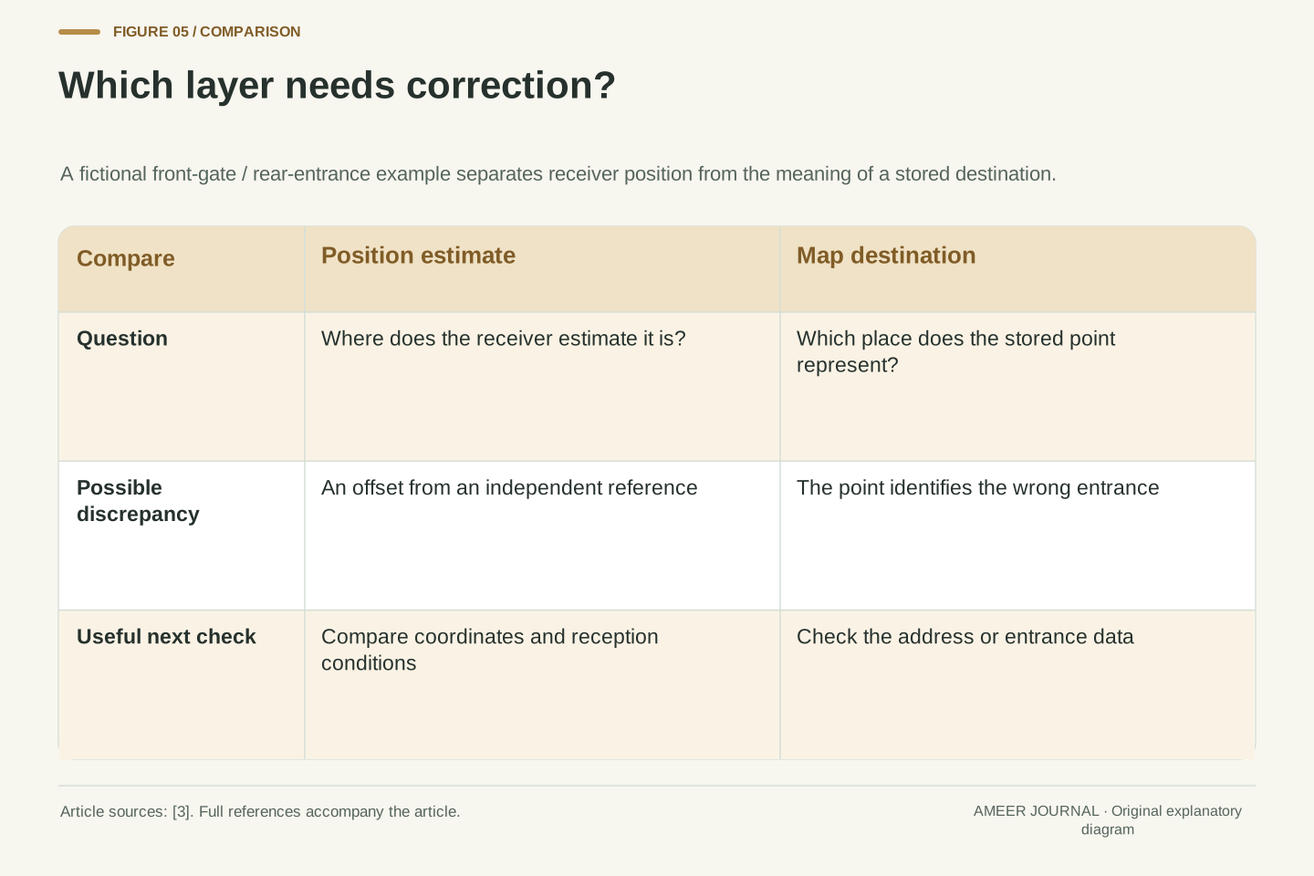
For a simple fictional case, imagine the receiver correctly places you at the front gate while the stored destination point is at the rear of the property. Improving the receiver's precision would not move that stored point to the front. Conversely, a perfectly placed map marker would not repair an offset receiver estimate. Keep those two possible corrections separate when describing what went wrong.
A useful report says which item appears wrong: your position, the named destination, the road drawing or the route instruction. Include the location and time where appropriate, without claiming to know the cause from the screen alone. That gives the relevant service a concrete problem to investigate. It also prevents a map-data issue from becoming an unsupported claim that all satellite navigation is inaccurate.
Coordinate estimation and geographic data interpretation are separate stages. GPS.gov explicitly identifies mapping-software problems as a source of apparent wrong-location behavior despite functioning positioning hardware. [3] Thus, evaluating a navigation application solely from the distance between a displayed destination and an expected entrance can confound receiver error with destination geometry or map-data semantics.
Consider a hypothetical correctly estimated front-gate coordinate paired with a database point representing a rear entrance. The mismatch is in the association between the user's task and the stored destination, not necessarily the position measurement. A tighter GNSS covariance would not correct that semantic mismatch. Conversely, accurate geographic data cannot eliminate a biased coordinate estimate. The example is a reasoning aid, not a reported incident.
When investigating, specify the object being evaluated and its reference. Is the comparison against the receiver's coordinates, an address point, a road centerline or an entrance? Preserve timestamp and coordinate-reference information if available, and avoid asserting a cause from one rendered map. A clearly defined discrepancy supports a useful next check; an undifferentiated screenshot of a misplaced dot usually leaves several explanations open.
Make a modest observation without inventing a benchmark
You can learn from a simple stationary observation, provided you keep its limits clear. In an ordinary safe location, note the time, surroundings and whatever position or quality information your device actually exposes. If you compare a more open location with one near a building, acknowledge that you also changed the place. GPS.gov identifies buildings and other obstructions as relevant, but a casual comparison does not isolate every cause. [3]
Separate what you saw from what you inferred. You might observe that dots spread more widely during one interval. That does not establish the absolute accuracy of either interval unless you have an independent reference. Write down missing information rather than filling it with guesses about satellite count, clock quality or an unseen processing algorithm.
Keep the original record if you later summarize it. State whether you examined raw coordinate outputs or only a displayed map, how long the observation lasted and what changed. This proposed exercise was not performed for the article. Its value is learning to ask a better question, not producing a laboratory-quality ranking from a few minutes beside a phone.
A useful exploratory record names the device, software or application context, timestamp, observable outputs and environmental conditions. If measurements from an open setting are compared with measurements near structures, preserve the fact that both location and reception conditions changed. GPS.gov supports obstruction as a plausible influence, not a causal diagnosis of an uncontrolled comparison. [3]
Distinguish a coordinate log from a rendered-map observation. Retain reported quality fields with their documented meaning if available, but do not invent access to diagnostics a device does not expose. Without a reference position, a set of repeated coordinates can characterize aspects of scatter, not establish absolute accuracy. Without controlled conditions, differences cannot be assigned uniquely to one receiver feature.
This is an observational method proposal rather than a completed experiment. Specify duration, sampling choices, excluded points and any visible interruptions before summarizing the data. If the application calls for a particular tolerance, the evaluation needs a reference and methodology suitable for that tolerance. The article's invented timing and coordinate examples supply no calibration, field validation or certification of any device.
Ask what the fix is good enough to decide
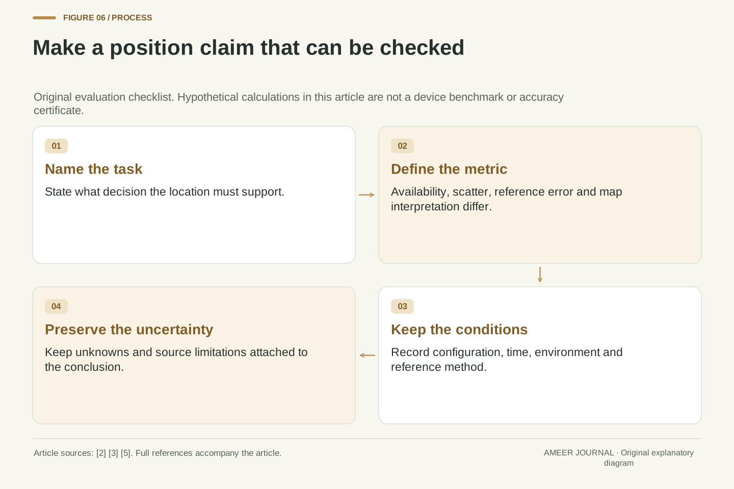
The useful question is not simply whether a receiver has found a location. It is whether the result supports your decision. Finding a meeting area, identifying the correct entrance and measuring a precise boundary demand different evidence. Start by naming the task, then ask what accuracy, update behavior and map information it requires. Do not borrow a precision claim made for different equipment or conditions.
When reading a specification or review, look for the measurement boundary: satellite signal quality, apparent range, calculated coordinates or the complete mapped route. Check the environment and the reference used to judge the result. GPS.gov's distinction between space-segment performance and user accuracy is a useful reminder that a favorable upstream number is not the entire story. [3]
A good explanation of a misplaced dot can now be more precise. The receiver may have a fix but uncertain geometry; repeated points may be tightly grouped yet offset; or the stored destination may be wrong. Keeping timing, estimation, accuracy and mapping separate makes the next check easier to choose. The coordinates remain useful, while the claim you make about them stays proportional to the evidence.
Define an acceptance criterion at the application boundary. Position availability, repeatability, horizontal or vertical accuracy, update behavior and correct destination interpretation are different requirements. A claim can satisfy one without satisfying the others. The receiver-state framework in ESA's introduction and GPS.gov's user-accuracy qualifications support keeping those requirements separate. [3][5]
For any quoted performance, record the evaluated quantity, reference, geometry or environment, receiver configuration and statistical meaning. An advertised ranging statistic is not a complete coordinate-error distribution. A sample mean is not an integrity bound. A highly repeatable display is not proof of a correct map. These distinctions are logical requirements for interpreting evidence, not additional measured performance claims.
The original examples deliberately establish only bounded conclusions: c converts timing to a range-equivalent scale; a shared clock parameter belongs in the position model; and a 0.71 m sample spread can coexist with an 8.63 m mean offset in the chosen dataset. Use the same discipline when updating an explanation for new equipment. Preserve the source scope, assumptions and unknowns rather than converting a new feature name or a successful fix into a universal accuracy promise.
Sources & further reading
Explore the references behind this guide. External pages may change after our review.
- How Does GPS Work? | NASA Space Place – NASA Science for KidsNASA Space Place · Accessed 6 Nov 2026
- GNSS Basic Observables - NavipediaEuropean Space Agency / Navipedia · Accessed 6 Nov 2026
- GPS Accuracy | GPS.govU.S. GPS program · Accessed 6 Nov 2026
- CODATA value: speed of light in vacuumU.S. National Institute of Standards and Technology · Accessed 6 Nov 2026
- GNSS Receivers General Introduction - NavipediaEuropean Space Agency / Navipedia · Accessed 6 Nov 2026
Article updated 6 Nov 2026.
Found something we should revisit?
Good explanations get better with thoughtful feedback.