What you’ll take away
- Induced emf depends on the negative rate of change of oriented flux linkage, not its value alone.
- In the specified fixed-field rotation, linkage extrema have zero emf while the zero crossings have voltage peaks.
- Equal flux values can accompany opposite voltages; even a known orientation needs the motion rate.
- The original quarter-turn has a 3 V endpoint emf but a time average of 6/π V, about 1.910 V.
- Changing the field changes the derivative, and a flux-only record does not complete a current, power or terminal-voltage model.
A large flux value does not say how fast it is changing
A coil can reach its largest magnetic flux while its induced voltage is momentarily zero. A quarter-turn later, its flux can be zero while the voltage is at a positive peak. Those statements sound contradictory only if flux and voltage are treated as two names for the same quantity. Faraday’s law relates an induced electromotive force, or emf, to how quickly the linked magnetic flux changes, rather than to the flux value alone [1].
Think of a graph with time along the bottom. The height of the flux graph tells you its value at a moment. Its slope tells you how quickly that value is changing. A smooth hilltop can have a large height and a flat tangent. A crossing through zero can have a steep tangent. The two readings answer different questions, even when they come from the same curve.
We will calculate a deliberately specified rotating coil, using ordinary wire-loop assumptions and a prescribed external field. Every number is an original teaching input, not a generator measurement. The exercise is a reading and calculation task: no coil, magnet, electrical connection or physical experiment is needed. The model lets us compare snapshots, directions and time intervals without guessing what an unspecified device would do.
For an ordinary material-wire circuit, the induction relation uses the time derivative of oriented flux, not its instantaneous magnitude [1][4]. For identical series turns, write the linked total as λ and the induced emf as ε=−dλ/dt. A value λ(t₀) is insufficient to determine that derivative. The distinction survives even when every geometric and field parameter is known except the motion history.
The main fixture is a rigid planar coil rotating smoothly in a spatially uniform, time-independent external magnetic field. Its rotation axis lies in the coil plane and is perpendicular to the field. Turns are identical and similarly oriented; their number is fixed. The field and motion are prescribed, with no load-dependent field or mechanical backreaction solved. These assumptions make the phase calculation explicit.
The original examples separate per-turn flux, linked total, emf, interval average and terminal/circuit interpretation. They do not represent a measured generator, motor-slip model or arbitrary current path inside an extended conductor. Feynman’s discussion specifically distinguishes the ordinary wire-loop rule from cases with changing material paths [4]. All numerical work below concerns the stated fixture and its separately declared variants.
Measure the angle from the surface normal
To describe the flux through one flat turn, first draw an arrow perpendicular to its surface. This is its chosen positive normal. In a uniform field, the flux depends on the field strength, the loop area and how closely that arrow points along the field [1][4]. The relevant angle is measured from the normal, not from the flat plane of the loop.
When the normal points along the field, the flux is positive and as large as it can be for those fixed field and area values. When the normal is perpendicular to the field, the flux is zero. When it points against the field, the flux is negative with the same largest magnitude. A negative value records orientation; it does not mean that the magnetic field strength has become negative.
Keep the normal attached to the coil as it rotates. Also declare a positive direction around the wire that agrees with it by the right-hand convention. These choices let a voltage sign mean something consistent from one position to the next. Reversing both conventions reverses the reported flux and emf signs without changing the physical arrangement or either magnitude.
Choose an oriented surface normal n and its associated positive circulation. Per-turn flux is Φ=∫B·n dA [1]. For a uniform field and planar area A this reduces to Φ=BA cos θ. In the rotating fixture, θ is a continuous rotation phase measured from alignment of n with B. It may run beyond π; it is not restricted to the unsigned principal angle between two vectors.
The dot product still gives the same cosine projection. At θ=0, Φ=BA; at π/2, Φ=0; at π, Φ=−BA. The first and third positions maximize the flux magnitude but have different signed values. Confusing the angle to the plane with the angle to its normal swaps the sine and cosine dependence and therefore misplaces the supposed voltage peaks.
Reversing the orientation convention sends n to −n and reverses positive circulation. Consequently Φ becomes −Φ and ε becomes −ε, preserving ε=−dΦ/dt. This is a relabelling, not a reversal of the actual rotation or field. The distinction matters when comparing signs across diagrams whose normal arrows or viewing directions differ.
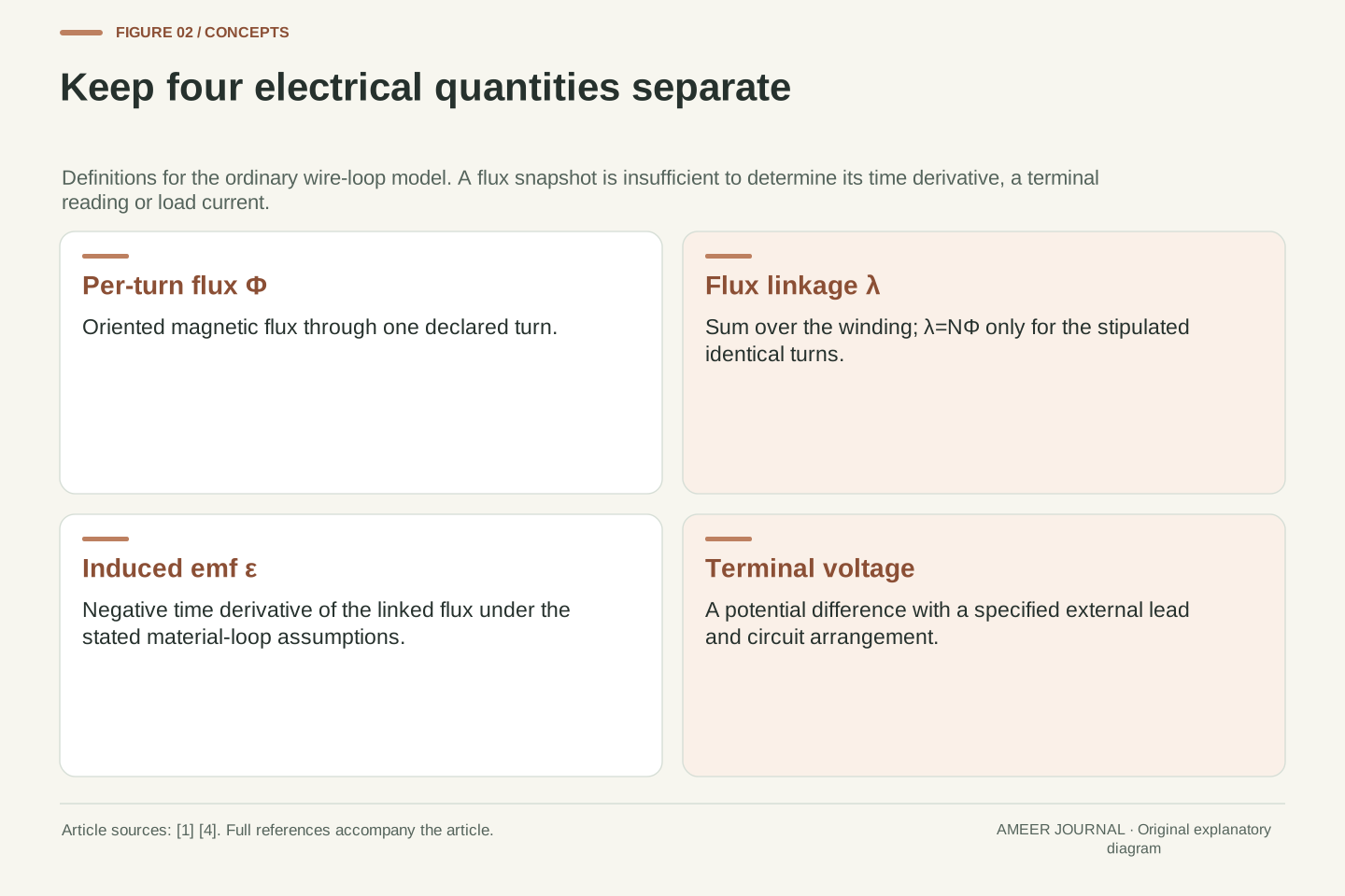
A per-turn flux and the linked total are different records
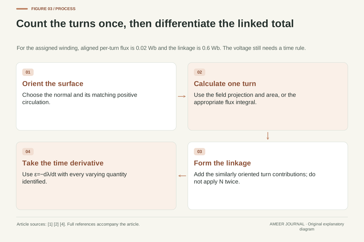
Use thirty identical turns, each with an area of 0.04 square metres, in a field of 0.5 tesla. These are assigned mathematical values. With the normal aligned to the field, the flux through one turn is 0.5 multiplied by 0.04, or 0.02 weber. The weber, abbreviated Wb, is the unit of magnetic flux; one weber equals one tesla times one square metre [1].
The same flux passes through each turn in this fixture. Adding the thirty similarly oriented contributions gives a linked total of 30 multiplied by 0.02, or 0.6 Wb. We call that total the flux linkage. The turn count has already been included in it. Multiplying by thirty again when calculating the coil’s emf would count the same turns twice.
A record should therefore say whether its flux number refers to one turn or the whole winding. Two reports labelled only flux could differ by a factor of thirty while describing the same coil. The multiplication rule also depends on the turns sharing the same flux and orientation [1]. Different areas, positions or winding directions need their actual contributions considered instead.
Let N=30, A=0.04 m² and B=0.5 T. The per-turn flux amplitude is BA=0.02 Wb. For the identical similarly oriented turns, λ=NΦ, so the linkage amplitude is Λ=NBA=0.6 Wb [1]. Turn count is dimensionless in SI; writing Wb·turn can help identify a linkage record, but it does not introduce a different physical dimension.
With constant N, ε=−d(NΦ)/dt=−N dΦ/dt=−dλ/dt [1]. The factor N appears once. If a supplied waveform already represents λ, applying another N would produce a thirtyfold overstatement for this fixture. This is a record-definition error, not a disagreement about the derivative operation or the magnetic-field unit.
For unequal linked turns, the corresponding oriented total is a sum of the individual fluxes, rather than an unexplained multiplication of one representative value. Our fixture avoids that extra distribution problem by stipulating identical exposure. Its numerical result therefore describes the assigned winding model; it does not establish the linkage of a real coil from a turn count alone.
The minus sign refers to change, not simply to field direction
Faraday’s law says to take the linked flux’s rate of change and reverse its sign [1]. If our linked total is increasing in the chosen positive direction, the induced emf is negative in the chosen circulation direction. If that same positive flux is decreasing, the induced emf is positive. The value can remain positive while the voltage changes sign.
Lenz’s law expresses the associated opposition to the change [2]. It does not say that an induced effect must always point against the existing field. In the familiar simple loop examples, an induced current can reinforce a field whose linked flux is falling. Which change is being opposed matters. The normal and circulation convention keep the mathematical sign separate from a loosely stated clockwise direction.
An emf is measured in volts, despite the historical word force in electromotive force [4]. In the flux rule, one weber of linkage change per second corresponds to one volt. The calculation needs both the amount of change and its timing. A linkage value of 0.6 Wb, by itself, supplies neither a voltage magnitude nor its sign.
The relation ε=−dλ/dt fixes the sign after the normal and positive circulation have been paired. Lenz’s law concerns opposition to the flux change, not unconditional opposition to B itself [2]. A positive λ can have positive, zero or negative slope; the corresponding emf signs are negative, zero or positive. The derivative requires a time-dependent record or an equivalent local motion/field specification.
Emf is the integrated tangential force per unit charge around the specified circuit, rather than a mechanical force measured in newtons [4]. Its SI unit is the volt. The induction relation is dimensionally ε in Wb/s, equal to V. Flux and voltage therefore cannot be interchanged numerically without a time scale, even before considering phase or sign.
The familiar opposition language is not a complete load solution. For example, inductive circuit response can retain current history even when the external induced emf passes through zero [4]. We calculate the externally prescribed induction contribution here, with no assumption that every actual current follows its sign instantaneously. A separate circuit model would be needed for that inference.
Give the coil a complete motion rule
Now let the normal start aligned with the field and rotate at five radians per second. A radian is an angle unit; a full turn contains two pi radians. The chosen rate therefore gives a full-turn time of two pi divided by five, about 1.257 seconds. The field strength, loop area and number of turns stay fixed throughout this main example.
For this rotation, the linked flux follows a cosine curve with a largest magnitude of 0.6 Wb. Differentiating it gives a sine-shaped emf whose largest magnitude is 0.6 multiplied by five, or 3 V. The constant-speed rotating-coil formulas are given in both the OpenStax generator discussion and Feynman’s generator analysis [3][4]. Our parameters and calculated values are independent teaching choices.
The rate is part of the explanation. Holding the coil still at a chosen orientation leaves its flux constant and gives zero emf from this fixed external field. Rotating it twice as fast through the same positions keeps the flux values at those positions but doubles their rates of change. The resulting voltage scale changes even though the geometric flux range does not.
Set θ(t)=ωt with ω=5 rad/s and t=0 at positive alignment. For fixed B, A and N, λ(t)=Λ cos(ωt)=0.6 cos(5t) Wb, with the trigonometric argument understood in radians. Differentiation gives ε(t)=Λω sin(ωt)=3 sin(5t) V [3][4]. The peak magnitude is 3 V and the period is 2π/5 s.
The phase relation follows from differentiation, not an extra delay element. The flux and emf have the same period, but their positive maxima occur a quarter-cycle apart. No assumption about current phase is included. The waveform is the prescribed coil’s induced emf; a circuit’s current and terminal response can require additional state variables and impedances.
More generally with fixed Λ, ε=Λ sin θ·dθ/dt. Constant ω is needed for this particular sine wave as a function of time, but not for that chain-rule identity [3]. A zero angular rate makes this contribution zero at any phase. Changing ω while keeping a particular orientation and field fixed changes ε without changing λ at that instant.
At the flux peak, the curve has a horizontal tangent
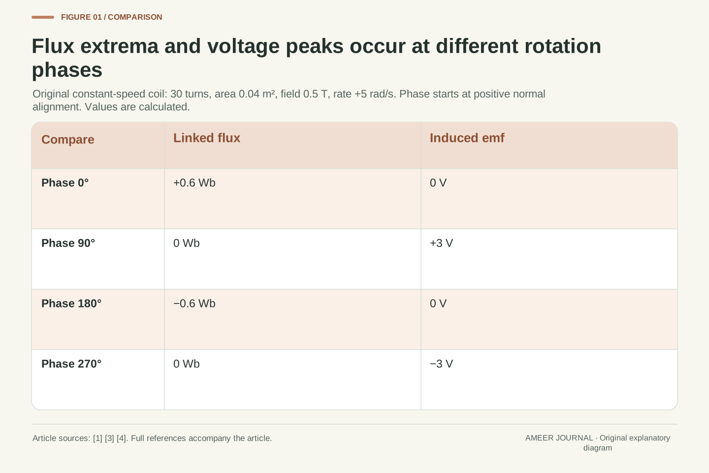
At the starting position, the linked flux is +0.6 Wb and the emf is 0 V. After a quarter-turn, the linked flux is zero and the emf is +3 V. After a half-turn, the linkage is −0.6 Wb and the emf is again zero. After three quarters of a turn, the linkage returns to zero while the emf is −3 V.
The zero at the start does not mean that the rotating coil is motionless. Near alignment, the cosine projection changes only slightly for a small angle change, and its instantaneous slope is zero at exact alignment. Near the quarter-turn position, the projection crosses zero most steeply under the assigned constant rotation. The flux’s height and slope reach their extremes at different positions.
This conclusion belongs to the specified smooth rotation with fixed field strength and area. It is not a rule that every moment of zero flux produces maximum voltage, nor that every aligned coil produces no voltage under any circumstances. We will change the motion and then the field to show why those broader interpretations fail.
At phases 0, π/2, π and 3π/2, the ordered linkage values are (0.6,0,−0.6,0) Wb and emf values are (0,3,0,−3) V. The derivative is zero at the smooth linkage extrema. At the zero crossings, its magnitude is Λω, giving the voltage peaks with the sign fixed by ε=−dλ/dt.
Around θ=0, cos θ has no linear term: its first change from unity is quadratic in a small phase displacement. Thus finite smooth angular velocity does not require a nonzero first time derivative at alignment. At θ=π/2, the cosine slope with respect to phase is −1, and multiplication by ω gives the largest negative linkage slope in this constant-speed fixture.
These are statements about the waveform and retained assumptions. They do not turn an orientation maximum at fixed B into a temporal maximum when B is changing. Nor does a single zero-crossing snapshot identify ω. The next comparisons hold the linked value fixed while changing the missing information that controls its derivative.
The same flux can accompany opposite voltages
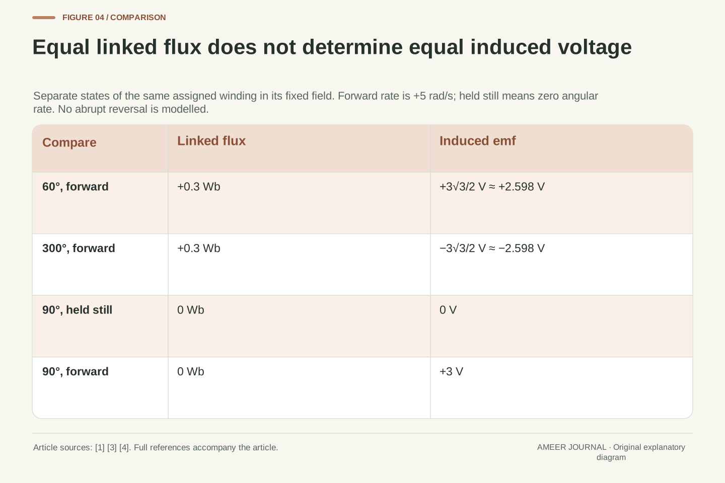
At a rotation phase of sixty degrees, the linked flux is +0.3 Wb. Later in the same forward rotation, at three hundred degrees, it is also +0.3 Wb. In the first position, the linked value is falling; in the second, it is rising. The induced voltages are therefore opposite: approximately +2.598 V and −2.598 V. Equal flux values have not fixed equal slopes.
Here phase means position within the declared full rotation, measured from the starting alignment. It keeps track of which side of that alignment the normal occupies. Both positions give the same projection onto the field, but the ongoing motion carries that projection in different directions. A picture that reports only the flux number discards that distinction.
There is an even simpler comparison at ninety degrees. A coil held there has zero linkage and zero emf from the fixed field. A coil passing the same orientation at five radians per second has zero linkage and +3 V emf. Reversing that rate at the same orientation gives −3 V. Position and motion must both be known.
For phases θ=π/3 and θ=5π/3 with ω=+5 rad/s, cos θ=1/2 in both cases. Hence λ=0.3 Wb, while sin θ=±√3/2 gives ε=±3√3/2 V, approximately ±2.598076 V. The pair uses different normals with the same field projection and the same forward angular rate.
A separate comparison holds the orientation itself fixed at θ=π/2. Rates dθ/dt of 0,+5 and −5 rad/s produce ε of 0,+3 and −3 V respectively, while λ remains zero in all three snapshots. These are separately declared local states, not an instantaneous physical reversal whose transient dynamics have been modelled.
The observations identify different missing variables. A flux value alone loses phase-branch information; even a known phase does not determine the angular rate. The signed formula ε=Λ sin θ·dθ/dt retains both. Magnitudes alone would additionally discard the sign of the induced emf, so an unsigned voltage plot cannot resolve the circulation direction.
An interval average is not the final voltage
The first quarter-turn takes pi divided by ten seconds, about 0.314 seconds. During it, the linked flux falls from 0.6 Wb to zero. The signed average emf equals the negative total linkage change divided by the elapsed time. That gives 0.6 divided by pi over ten, or six divided by pi: approximately 1.910 V.
The voltage at the end of that interval is 3 V. These results differ because the voltage was not 3 V throughout the quarter-turn. It began at zero and increased along a sine curve. Using the final value for the entire interval would overstate the integrated voltage. The finite-interval calculation follows by integrating the same derivative relation used for the instantaneous waveform [1][4].
Averaging just the starting and ending readings would give 1.5 V, which is also different from 1.910 V. That shortcut would be exact for a voltage changing linearly with time across the interval; our sine curve does not. State the interval and the averaging rule instead of treating a peak, an endpoint average and a time average as interchangeable.
For t₁=0 and t₂=π/10 s, Δλ=−0.6 Wb. Integrating ε=−dλ/dt gives ∫ε dt=−Δλ=0.6 V·s. Therefore the time mean is ε̄=−Δλ/Δt=6/π V≈1.909859 V. This is an original calculation from the derivative identity, independent of a sampled endpoint approximation [1][4].
At t₂, ε=3 V. The ratio of the interval mean to this peak is 2/π≈0.636620. Direct integration of 3 sin(5t) over the same interval reproduces 0.6 V·s. The quarter-turn duration and linkage endpoints must refer to the same motion; mixing the duration from one angular rate with the endpoint voltage from another would define a different calculation.
The arithmetic mean of the two endpoint voltages is (0+3)/2=1.5 V. It is the trapezoidal estimate for this interval, not the exact sine-wave mean. Neither 1.5 V nor 3 V should be labelled the exact quarter-turn average. The distinction is between instantaneous differentiation and finite-interval integration, not between two competing versions of Faraday’s law.
A zero signed average does not mean nothing happened
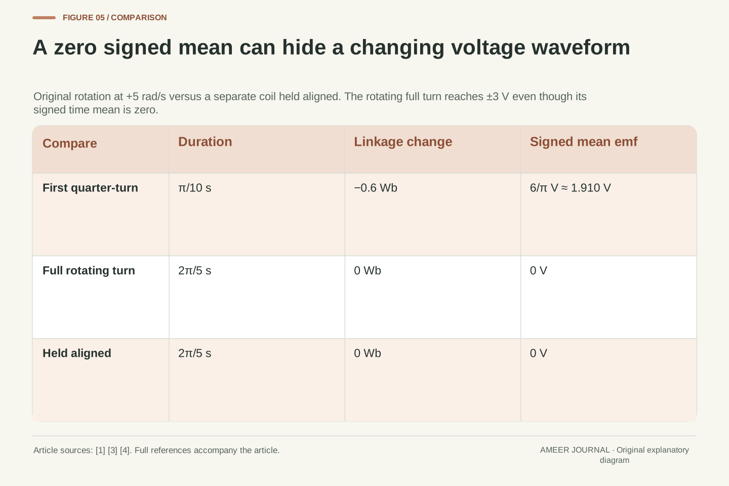
After one complete turn, the linked flux returns to +0.6 Wb. Its total change is zero, so the signed average emf over that whole turn is zero. Yet the waveform reached +3 V and −3 V along the way. Positive and negative contributions cancel in the signed time total; the individual voltage values do not disappear.
Compare a separate coil held still at the starting alignment for the same duration. Its linked flux also begins and ends at +0.6 Wb, and its average emf is also zero. This time the emf remains zero throughout. Identical endpoint flux records and identical elapsed times therefore leave different possible voltage histories between those endpoints.
If we average voltage magnitude instead, the full rotating turn gives about 1.910 V rather than zero. That is another named calculation, using positive sizes instead of signed values. Neither average alone determines electrical energy delivered to a load: that also involves current [4]. The record must identify whether it contains signed emf, magnitude, a peak or a circuit power quantity.
Over T=2π/5 s, λ(T)=λ(0)=0.6 Wb and ∫₀ᵀ ε dt=0. Hence ε̄=0. The same endpoints and duration occur for a separately stationary aligned coil with ε(t)=0 throughout. The rotating and stationary histories demonstrate that an endpoint difference determines the signed integral, not the internal waveform.
For the rotating sine wave, ∫₀ᵀ |ε|dt=4Λ=2.4 V·s. Dividing by T gives the mean magnitude 6/π V≈1.909859 V. The coincidence with the first-quarter signed mean follows from this symmetric sinusoid; it is not an identity for arbitrary waveforms or arbitrary averaging windows.
Voltage-time integral is not electrical energy. The generator power expression also contains current, εI [4]. Consequently ∫ε dt=0 does not establish ∫εI dt=0, and the present flux-only record supplies no actual load energy. Keeping the signed integral, magnitude average and power integral distinct prevents cancellation in one quantity from being transferred to another.
An aligned coil can still have emf if the field changes
The flux peak statement depended on a fixed field. For a separate case, hold the same coil aligned and stationary while its uniform field increases at 0.2 tesla per second. At the moment the field is 0.5 tesla, the linked flux is again +0.6 Wb. Its rate of change, however, is thirty times 0.04 times 0.2, or +0.24 Wb per second.
Faraday’s law gives an emf of −0.24 V in the chosen direction. Alignment maximizes the flux for the field strength present at that moment, but the field itself is growing. The linked flux is therefore not at a time maximum. This case explains why maximum possible at a fixed field and maximum along a time record must not be treated as the same statement.
Changing area would introduce another way for the flux to change [1]. The useful habit is to identify everything allowed to vary before differentiating. In our rotating example only orientation changed; in this new stationary example only field strength changes. Holding those cases apart makes the differing voltage results consistent rather than contradictory.
For a separate stationary aligned state, keep N=30 and A=0.04 m², with B(t)=0.5 T+(0.2 T/s)t near t=0. Then λ(t)=0.6 Wb+(0.24 Wb/s)t and ε=−0.24 V. At t=0, λ equals the main fixture’s positive peak value, but its derivative is nonzero. The comparison changes a declared input, not the induction relation.
With fixed N but uniform B(t), area A(t) and phase θ(t), the product/chain rule gives ε=−N[A(dB/dt)cos θ+B(dA/dt)cos θ−BA sin θ(dθ/dt)]. This expression assumes the stated uniform planar geometry; the general nonuniform case returns to the flux integral [1]. The main rotating model retains only its last term.
At alignment, the angular term vanishes, but the field-rate or area-rate terms need not. An orientation extremum at fixed parameters is therefore different from a temporal extremum when those parameters evolve. This is also why a claim about induced emf should carry the fixed-field, fixed-area assumptions beside its phase argument.
The coil calculation does not complete the circuit description
The quantity we calculated is the coil’s induced emf. A terminal voltage reading also needs a defined arrangement of leads and circuit connections. Feynman’s generator discussion states a particular no-load case: where the outgoing wires are in a suitable region without a changing magnetic field, their potential difference equals the rotating coil’s emf [4]. That is a qualified connection, not permission to ignore measurement geometry everywhere.
Current needs further information. A simple resistance-only model relates current to emf through resistance, but real circuit descriptions can include inductance and other components. The same source explains how a coil’s own changing current contributes another induced emf [4]. An instantaneous zero in our external induction waveform does not, by itself, prove that every possible connected circuit has zero current then.
These extra relationships also matter for power and mechanical loading. A large induced voltage is not an efficiency measurement or a complete output-power rating. Our example keeps the field and motion prescribed so that the flux derivative can be examined cleanly. Its record contains no measured load, current, winding loss or actual machine operating limit from which those further results could be calculated.
The emf around a specified moving wire circuit is not automatically a globally defined electrostatic potential difference. Feynman’s generator analysis supplies a no-load terminal interpretation in a suitable external region where the electric field admits a potential [4]. Our winding calculation does not specify arbitrary lead loops, contact geometry or a measurement instrument’s complete coupling to the field.
Nor is ε(t) alone a current solution. Under a separately stipulated resistance-only approximation one could use I=ε/R, whereas inductive state introduces additional time dependence. Feynman explicitly treats the self-induced contribution −L dI/dt under a consistent sign convention [4]. No L, resistance, initial current or external circuit is supplied by the present main fixture.
The given external field and angular motion therefore determine the stated induction waveform without certifying delivered power, efficiency or load-dependent operation. Those quantities require an enlarged model and evidence. The distinction lets the elementary derivative result remain useful without silently treating a prescribed-source calculation as a complete generator test.
Keep the value, the time rule and the requested quantity together
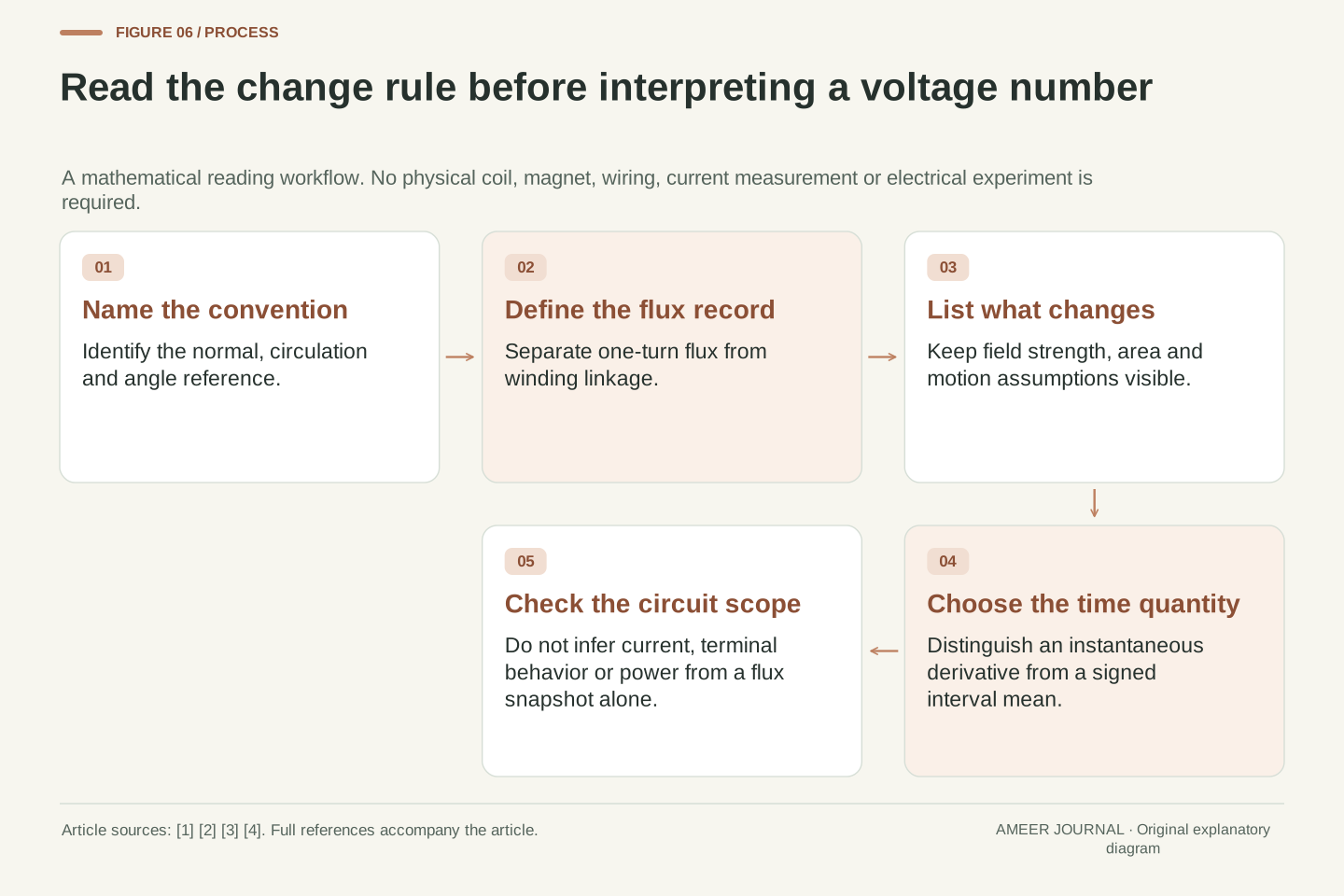
When reading a coil diagram, begin with the normal arrow and the meaning of its angle. Then identify whether the reported flux belongs to one turn or the whole winding. State which field, area and motion quantities stay fixed. This small record is enough to prevent several different mistakes before any arithmetic begins.
Next ask which voltage quantity is wanted. At one moment, use the local rate of linkage change. Across an interval, use the negative endpoint change divided by the duration for the signed mean. For the original first quarter-turn, these give 3 V at its endpoint and about 1.910 V as its time average. The names keep both correct values attached to their questions.
Finally, keep circuit questions separate from flux snapshots. Our thirty-turn example can have linkage 0.6 Wb with zero emf during fixed-field rotation at alignment, or −0.24 V in the separately increasing-field case. It can also have zero linkage with zero, positive or negative emf depending on motion. The missing information is the change rule, not another guess about the size of the flux.
A reproducible induction record identifies the oriented surface and circulation, turn linkage definition, field distribution, geometry and time-dependent variables. For the constant-speed fixture, retain N,A,B,ω and initial phase. If the field or area varies, preserve those functions or local derivatives instead of reusing the fixed-parameter sine law without its conditions.
Choose the requested functional before calculating: instantaneous ε=−dλ/dt, signed interval mean −Δλ/Δt, mean magnitude, or a circuit-dependent quantity involving current. These are different operations on the available record. Our exact quarter-turn integral, full-turn cancellation and stationary comparison demonstrate why endpoint flux data cannot reconstruct every internal voltage history.
The central inference is narrow and useful: a linked-flux value is not its derivative. Equal values can accompany opposite slopes, and an orientation maximum can coexist with nonzero emf when another parameter changes. Once those missing variables and conventions are explicit, the original phase and interval calculations agree without requiring invented measurements or a universal claim about all motors and generators.
Sources & further reading
Explore the references behind this guide. External pages may change after our review.
- 13.1 Faraday’s Law - University Physics Volume 2 | OpenStaxOpenStax / Rice University
- 13.2 Lenz's Law - University Physics Volume 2 | OpenStaxOpenStax / Rice University
- 13.6 Electric Generators and Back Emf - University Physics Volume 2 | OpenStaxOpenStax / Rice University
- The Feynman Lectures on Physics Vol. II Ch. 17: The Laws of InductionThe Feynman Lectures on Physics / California Institute of Technology
Article updated 7 Nov 2026.
Found something we should revisit?
Good explanations get better with thoughtful feedback.