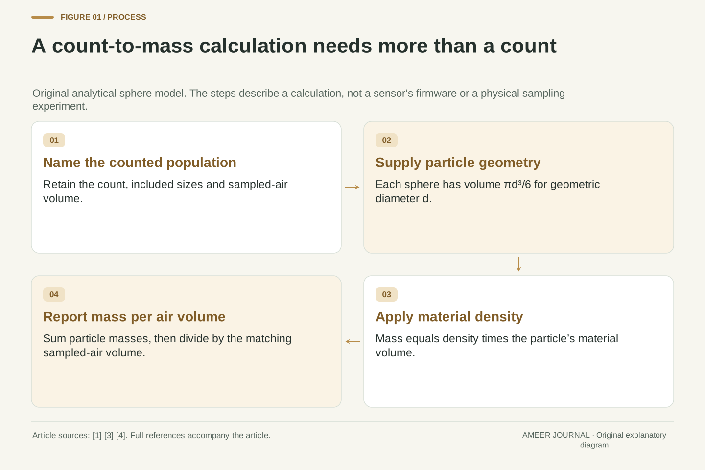
An air sensor can report how many particles it detects, or an estimate of particle mass in a volume of air. Those quantities are related, but there is no universal multiplier that converts one into the other. The particles’ sizes and material matter. A hundred large particles can carry more mass than several hundred smaller ones, even when both populations occupy the same amount of air.

EPA’s sensor tables distinguish optical counting, light-scattering measurements and estimated mass outputs [3]. CARB separately describes weighing collected particulate material and using scattered light to estimate particle number and size [4]. A displayed mass number therefore needs its measurement method and interpretation; its units alone do not reveal how the number was obtained.

We will use original numerical populations of uniform spheres to make the conversion transparent. Their geometric sizes, densities and air volumes are supplied exactly. No air is sampled and no sensor is tested. The exercise will show what information a count omits, why an average diameter may still be insufficient, and how overlapping size counts can accidentally count the same particle more than once.

Particle number concentration and particle mass concentration are different moments of a size-and-material population. NASA’s aerosol description distinguishes number, area and volume distributions and notes that a density assumption is needed to relate volume to mass [1]. EPA and CARB distinguish optical particle measurements from gravimetric mass measurements [3][4].

The original fixture assumes homogeneous spheres with assigned geometric diameters, specified material densities and known sampled-air volumes. Counting is ideal and complete within each declared included population. These are analytical inputs, not measured optical-equivalent diameters, a sensor-efficiency model or a reconstruction of proprietary firmware. Exact Fraction arithmetic checks the rational coefficients; displayed π-dependent values are rounded.

The central question is which additional information converts number into mass. We will distinguish raw count from concentration, volume weighting from count weighting, mean diameter from mean cubed diameter, and cumulative thresholds from disjoint bins. No aerosol generation, instrument trial, exposure assessment, air-quality-index calculation, regulatory determination or product recommendation is made.

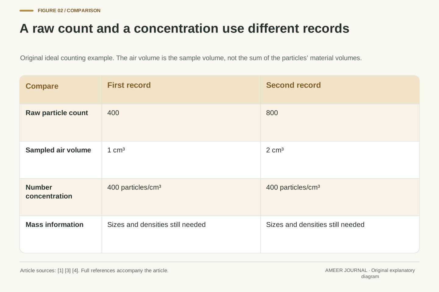
Suppose an ideal record contains 400 particles in one cubic centimetre of air. Another contains 800 particles in two cubic centimetres. The second count is twice as large, but both number concentrations are 400 particles per cubic centimetre. Dividing by the sampled air volume makes the records comparable. Looking only at the two raw counts would miss the changed denominator.

A cubic centimetre here measures the air sample, not the volume occupied by solid particles. The particles occupy only part of that space. Later, we will also calculate the particles’ own volumes, so keeping those two meanings of volume separate is essential. More air sampled and larger individual particles are different changes.

A real comparison also needs compatible sampling periods and included size ranges. EPA’s table definitions explicitly distinguish detection approach, data units and averaging or testing intervals [3]. Our ideal records have supplied the complete population and air volumes. They do not assume that a real instrument detects every particle or measures every possible size.

Let N denote the number of included particles and V_air the sampled-air volume. Number concentration is n=N/V_air. The two assigned records give 400/1=800/2=400 cm⁻³. N is a count; n carries an inverse-volume unit. A different sampling volume can therefore change N without changing n.

V_air is distinct from the summed material volume of the particles. That distinction will remain explicit when particle geometry enters the mass calculation. The denominator refers to the air containing the population, while a sphere’s volume refers to the material inside that sphere. Neither quantity should silently replace the other.

The records assume complete counting of a known included set over their declared sampling intervals. Real collection and detection efficiencies are not supplied. EPA identifies output units, averaging times, test intervals and detection mechanisms as separate fields in sensor evaluations [3]. A raw event count without a matching air volume and selection boundary cannot establish the same concentration comparison as our fully specified records.

Imagine a spherical particle with a diameter of one micrometre. A micrometre is one-thousandth of a millimetre. If another sphere has half that diameter, it has half the width in each of three dimensions. Its volume is one half times one half times one half, or one eighth as large. At equal material density, its mass is also one eighth as large.

An exact numerical description uses sphere volume equal to π times the diameter cubed, divided by six. Density then converts that material volume into mass. NASA’s volume-distribution equation uses the corresponding radius-cubed weighting [1]. Radius is half the diameter; putting a diameter directly into a radius formula would make the calculated volume eight times too large.

Our next records use diameter in micrometres and material density in grams per cubic centimetre. The final mass concentration will be in micrograms per cubic metre of air. Those unit changes are part of the calculation. They do not mean that a micrometre-sized sphere fills a cubic metre of air.

For a sphere of geometric diameter d, radius r=d/2 gives V_particle=4πr³/3=πd³/6. The native NASA volume-distribution equation retains the 4π/3 radius-cubed factor [1]. Multiplying by uniform material density ρ gives m_particle=ρπd³/6 in consistent units. The cubic dependence is geometric, not an empirical optical-response law.

With d entered numerically in µm and ρ in g/cm³, convert d using 1 µm=10⁻⁴ cm. Then m_particle=ρπd³·10⁻¹²/6 g, or ρπd³·10⁻⁶/6 µg. A one-micrometre, unit-density sphere therefore has mass π/(6×10⁶) µg. This tiny single-particle mass is not yet an air concentration.

Number concentration in cm⁻³ converts to m⁻³ by multiplying by 10⁶. Thus for a single-size population, the numerical mass concentration in µg/m³ is nρπd³/6 when n, ρ and d use those exact stated units. The cancelling powers of ten do not authorize mixing other units into the same numerical expression.

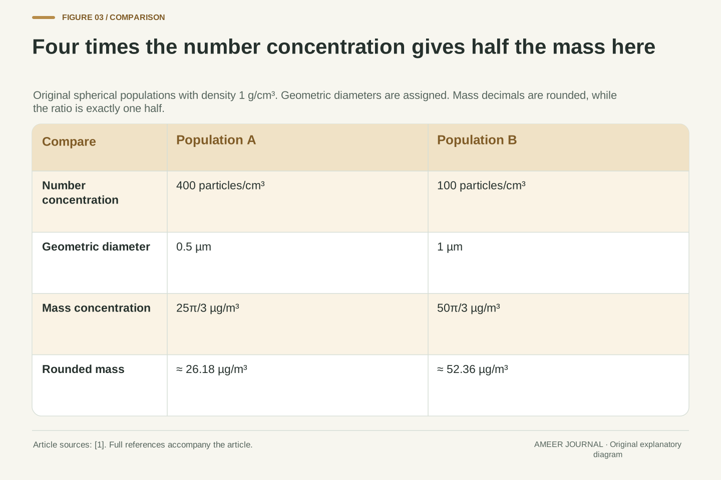
Give population A 400 particles per cubic centimetre, each 0.5 micrometres in diameter. Give population B 100 particles per cubic centimetre, each one micrometre in diameter. All particles are spheres with the same assigned density of one gram per cubic centimetre. A has four times B’s number concentration.

Each A particle, however, has one eighth the mass of a B particle. Combining the count and individual-mass comparisons gives four times one eighth, or one half. A’s particle mass concentration is about 26.18 micrograms per cubic metre, while B’s is about 52.36. More particles has coincided with less mass in this fully specified comparison.

The result does not depend on rounding those two displayed mass values. The exact ratio is one half because the shared density and sphere factor cancel. NASA notes that relatively few coarse particles can account for much of an aerosol’s mass or volume [1]. Our assigned populations demonstrate the weighting principle without claiming to reproduce any particular atmospheric sample.

Assign A: n_A=400 cm⁻³, d_A=1/2 µm, ρ_A=1 g/cm³. Assign B: n_B=100 cm⁻³, d_B=1 µm, ρ_B=1 g/cm³. Their mass concentrations are M_A=400·(1/2)³π/6=25π/3 µg/m³≈26.17994 µg/m³ and M_B=100π/6=50π/3 µg/m³≈52.35988 µg/m³.

Although n_A/n_B=4, the individual sphere-mass ratio is (d_A/d_B)³=1/8. Therefore M_A/M_B=4/8=1/2. These are exact ratios within the assigned equal-density sphere model; only the π-dependent decimal displays are rounded. The air-volume convention is identical across the two populations.

This is a direct counterexample to inferring a mass ordering from a number-concentration ordering alone. The general source distinction between number and volume weighting supports the interpretation [1]. No particle composition, sensor response or health ranking follows from the two numerical mass concentrations. The known geometry supplies the missing conversion information that an unqualified count would lack.

Now make a separate mixed population in one cubic centimetre of air. It contains ninety spheres of diameter 0.5 micrometres and ten spheres of diameter two micrometres. All have the same density. The larger group is only ten out of one hundred particles, so its share of the count is ten percent.

For mass, weight each count by the diameter cubed. The smaller group contributes 90×0.5³=11.25 comparison units. The larger group contributes 10×2³=80. Together they give 91.25. The larger group therefore supplies 80 divided by 91.25, about 87.67 percent of the mass. Its ten-percent count share and its much larger mass share describe the same population.

The comparison units omit the common density and sphere-volume factor, which cancel when taking a share. They are not measured micrograms. A chart showing the percentage of particles in each size group can consequently look very different from a chart showing the percentage of mass, even when both use exactly the same underlying particles.

For an independent equal-density population, take n_s=90 cm⁻³ at d_s=1/2 µm and n_l=10 cm⁻³ at d_l=2 µm. The large-particle number fraction is n_l/(n_s+n_l)=1/10. The diameter-cubed contributions are 90/8=45/4 and 80, totaling 365/4 in the common numerical unit convention.

The large-particle mass fraction is therefore 80/(365/4)=64/73≈0.8767123. The small-particle mass fraction is 9/73. Common ρπ/6 factors cancel in these fractions, but the d³ weights do not. This is the kind of difference between number and volume distributions discussed by NASA [1], instantiated here with original finite records.

The denominator must be named before interpreting a size-bin percentage. A number-normalized histogram sums counts; a mass-normalized histogram sums mass contributions. Equal bin labels do not make their vertical axes equivalent. The example also does not assert that the group with the most mass dominates every optical measurement, since optical response depends on properties beyond this mass weighting.

Return to population B, with one hundred one-micrometre spheres per cubic centimetre. Keep those sizes and the count, but assign a material density of two grams per cubic centimetre instead of one. The total particle volume stays the same. The calculated mass doubles, from about 52.36 to 104.72 micrograms per cubic metre.

Density tells us how much mass occupies a unit of the particle material’s volume. It is not the number of particles packed into the air sample. Doubling number concentration and doubling material density can both double this model’s mass concentration, but they change different parts of the record. One changes how many spheres there are; the other changes the mass of each sphere at the same size.

NASA’s discussion makes the mass–volume connection conditional on density [1]. Our comparison has supplied that density directly. It does not say that changing material would leave scattered light unchanged or that an optical sensor could identify the new density from its count alone.

Hold B’s n=100 cm⁻³ and d=1 µm fixed while assigning ρ=2 g/cm³. Then M=100·2π/6=100π/3 µg/m³≈104.71976 µg/m³, exactly twice the unit-density result. The total geometric particle volume per air volume is unchanged; the mass per material volume has changed.

For multiple size or material classes, the general discrete expression is M=Σn_jρ_jπd_j³/6 under the stated numerical units. Factoring out a common density is justified only when the included classes share that density. A count and size distribution without density information does not uniquely determine this mass account [1].

This comparison is a geometric/material calculation, not a scattering invariance experiment. Refractive index, shape and other optical properties could differ between real materials [4]. We make no claim that two equal-size populations of different densities would produce the same optical signal. Keeping the measured or assumed quantities distinct prevents the algebra from overstating what one detector channel can identify.

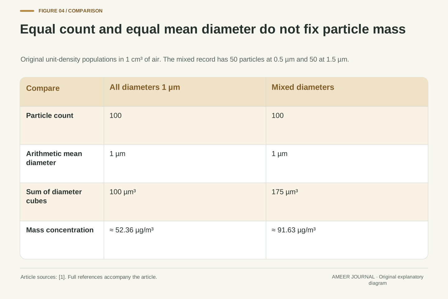
Could a count plus an average diameter solve the problem? Consider two more records, each with one hundred spheres per cubic centimetre and density one. The first is B: every diameter is one micrometre. The second has fifty particles of diameter 0.5 and fifty of diameter 1.5 micrometres. Both arithmetic mean diameters are one micrometre.

Their mass totals differ. B’s sum of cubed diameters is one hundred. The mixed record gives 50×0.5³+50×1.5³=6.25+168.75=175. With the same density, the mixed population has 1.75 times B’s mass concentration: about 91.63 rather than 52.36 micrograms per cubic metre.

The average diameter has hidden the spread between smaller and larger particles. Cubing the average before doing the mass calculation would give the all-one-micrometre answer for both records. It would miss the larger particles’ heavier contribution. A useful average must retain the particular weighting needed for the question; the word average by itself does not specify that weighting.

Compare B with a mixed record having 50 cm⁻³ at d=1/2 µm and 50 cm⁻³ at d=3/2 µm, all at ρ=1 g/cm³. Both have n=100 cm⁻³ and number-weighted arithmetic mean diameter d̄=1 µm. However, their sums Σn_jd_j³ are 100 and 175 in the declared numerical convention.

The mixed mass concentration is 175π/6 µg/m³≈91.62979 µg/m³, so M_mix/M_B=175/100=7/4. Equal number concentration and equal first-moment mean do not identify the third-moment quantity needed for spherical mass at common density. NASA distinguishes size-distribution moments and their volume-weighted counterparts [1].

This counterexample requires no fitted probability distribution, random sampling or uncertainty estimate. The finite population is specified exactly. The result is about information lost by replacing the individual diameters with their arithmetic mean; it is not evidence of bias in a tested instrument. Additional distribution information is necessary to distinguish these two accounts.

For the mixed record, divide the sum of cubed diameters, 175, by the one hundred particles. The average cubed diameter is 1.75 cubic micrometres. The cube of the average diameter is only one cubic micrometre. Those two calculations use the same diameters in a different order, and they produce different answers.

We can define another diameter: the size of a sphere whose volume equals the average particle volume in this model. Its cube must be 1.75, so its diameter is about 1.20507 micrometres. This is larger than the arithmetic mean diameter of one micrometre. It does not mean every particle has become 1.20507 micrometres wide; it is a chosen summary of their average volume.

Before using a reported mean size, ask how it was calculated. A mean weighted by number, a mean weighted by mass and a diameter chosen to match average volume need not agree [1]. Our two means are derived from the declared geometric sizes, not from an optical sizing algorithm.

For the mixed fixture, the number-weighted mean cube is E_N[d³]=175/100=7/4 µm³, whereas (E_N[d])³=1 µm³. Here E_N means the exact average across the stated finite number distribution, not an expectation estimated from random observations. The mass account uses E_N[d³], since M is proportional to nρE_N[d³].

Define a volume-equivalent mean diameter d_v=(E_N[d³])^(1/3). It is (7/4)^(1/3) µm≈1.20507 µm in this fixture. At common density, a sphere of this diameter has the average particle mass. It is a different statistic from d̄ and does not identify either actual diameter in the two-size mixture.

The source’s distinction between number and volume moments supports keeping such summaries separate [1]. This article does not use the surrounding lognormal-distribution formulas or assume a lognormal fit. Nor does it identify d_v with an aerodynamic or optical-equivalent diameter. The original expression states exactly which average has been taken and which geometric relationship gives it meaning.

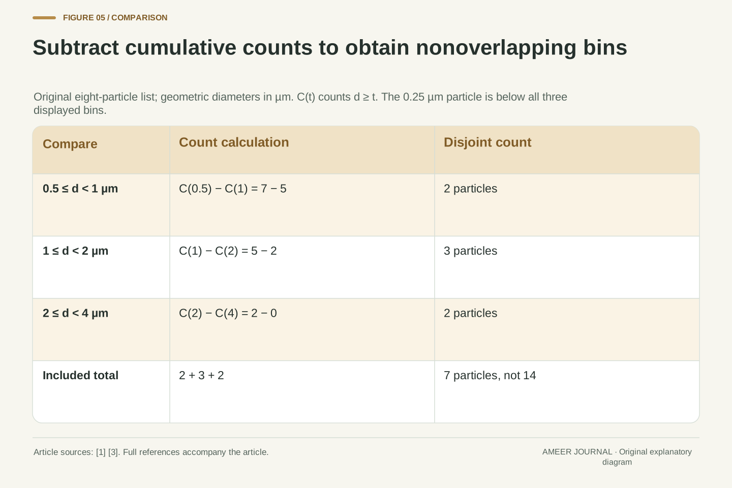
Size labels can hide another problem. Make a record of eight particles with diameters 0.25, 0.5, 0.75, 1, 1.25, 1.5, 2 and 3 micrometres in one cubic centimetre. Define each threshold to include particles equal to or larger than its label. The counts at thresholds 0.5, 1, 2 and 4 are seven, five, two and zero.

Adding seven, five and two gives fourteen, although only seven particles meet the lowest threshold. The same particles have been counted in several overlapping groups. In particular, the two particles at 2 and 3 micrometres belong to all three nonempty threshold groups.

Subtract neighboring cumulative counts instead. The interval from 0.5 up to but not including 1 contains 7−5=2 particles. The interval from 1 up to 2 contains 5−2=3. The interval from 2 up to 4 contains 2−0=2. These three nonoverlapping counts sum to seven. The particle at 0.25 is outside all three included intervals.

For the exact geometric diameters (0.25,0.5,0.75,1,1.25,1.5,2,3) µm, define C(t)=#{d_i≥t}. Then C(0.5)=7, C(1)=5, C(2)=2 and C(4)=0. These are cumulative counts for a one-cubic-centimetre air record, not disjoint-bin frequencies. Their sum 14 double-counts membership.

Differences form half-open bins: C(0.5)−C(1)=2 for [0.5,1), C(1)−C(2)=3 for [1,2), and C(2)−C(4)=2 for [2,4), with bounds in µm. Each included particle belongs to exactly one bin; the 0.25 µm particle is excluded. The inclusive cumulative convention determines where boundary particles enter.

EPA’s tables include cumulative particle counts and size-range outputs [3], but the thresholds and ≥ convention here are independently declared. They are not copied from a device’s greater-than channel specification. A real channel record must retain its own endpoint and detection convention before any subtraction or mass conversion is applied.

The top interval in our record contains two particles, one at 2 micrometres and one at 3. Each contributes one to the count. In the equal-density sphere account, their diameter-cubed weights are eight and twenty-seven. Treating them as equal-mass particles merely because they share a bin would discard information we already have.

For all seven included particles, the sum of cubed diameters is 41.875 in cubic-micrometre units. That sum can be calculated because this record supplies every diameter. If only the three bin counts—two, three and two—were available, the exact same sum would not follow. Different positions within the allowed intervals could preserve those counts while changing the mass.

A conversion that represents every particle in a bin by one chosen size therefore introduces an approximation or model assumption. Its result needs that choice recorded. The bin’s label does not prove that all particles sit at its midpoint, and an open-ended top bin would not even supply a finite upper endpoint from which to form a midpoint.

Within [2,4) µm, the two actual diameters 2 and 3 contribute d³ values 8 and 27 µm³. Their equal count weights therefore differ substantially from their equal-density mass weights. For the seven particles with 0.5≤d<4 µm, the exact sum is Σd_i³=335/8=41.875 µm³.

At unit density in the one-cubic-centimetre air sample, their mass concentration is consequently (335π/48) µg/m³. This follows from the complete diameter list, not solely from the three counts (2,3,2). Retaining only counts within finite intervals leaves the within-bin third moment unidentified. Changing a diameter inside its interval can change that moment without changing any cumulative count.

A representative-diameter conversion closes this missing information by assumption. It can be an intentionally chosen approximation, but should not be presented as an exact consequence of bin totals. The distinction also separates our transparent sphere account from a sensor’s calibrated inference method [3][4]. No proprietary bin conversion or optical inverse problem is reproduced here.

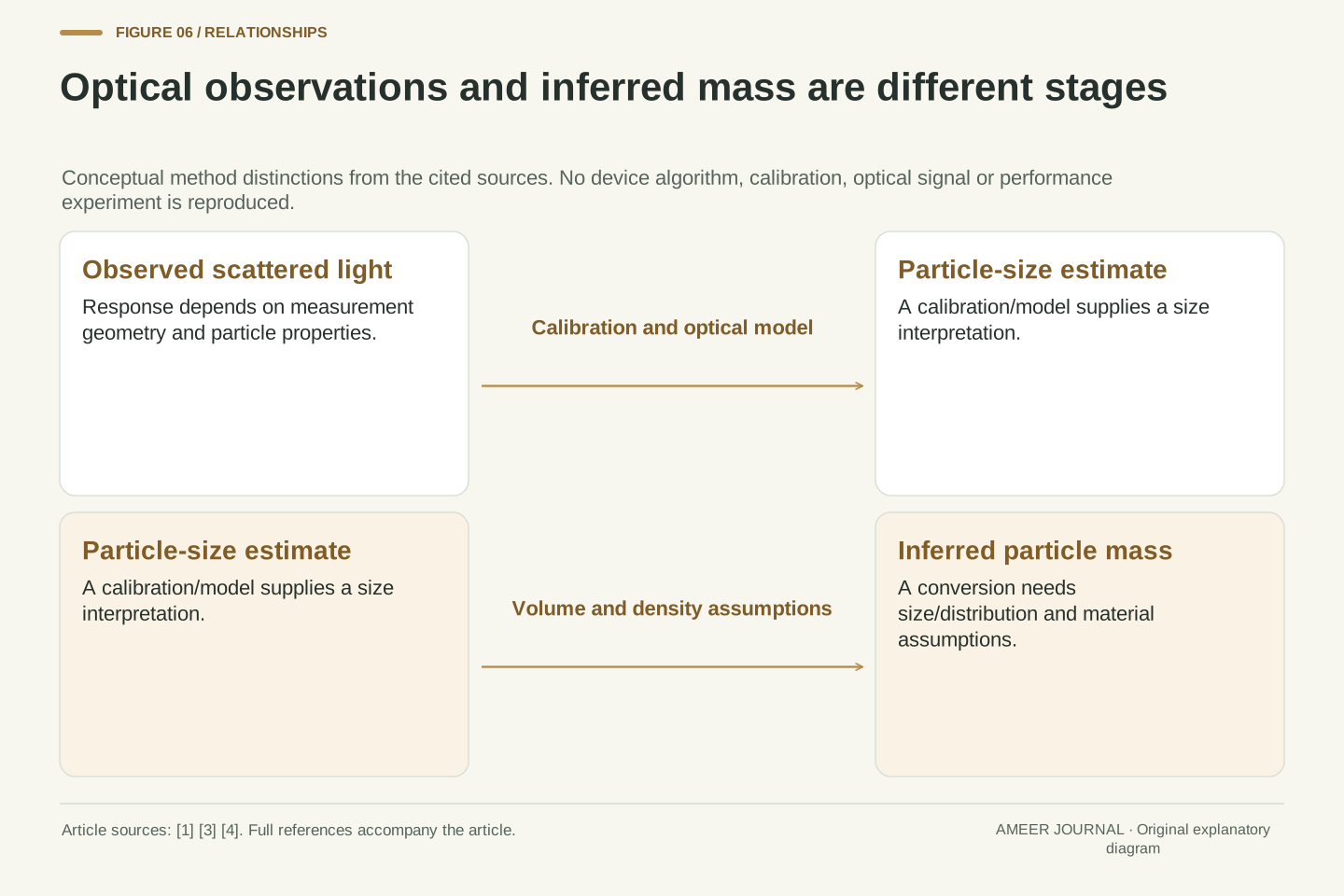
So far, every diameter has been given to us. An optical particle counter faces another task: it observes scattered light and uses a calibration and measurement model to estimate particle number and size. CARB describes this process and notes that particle shape and refractive index affect the scattering response [4]. NASA also identifies wavelength, size distribution and composition as relevant to aerosol scattering [1].

A mass estimate built from optical observations therefore carries assumptions before the diameter-cubed calculation even begins. It is not simply a balance weighing every particle. CARB describes a different approach in which collected particle mass is related to the volume of air sampled [4]. EPA’s table also distinguishes an instrument with an integrated collection filter from its optical measurement [3].

These differences do not establish that one unnamed sensor is wrong. They explain why agreement depends on what was measured, how the output was derived and which conditions were compared. Our arithmetic tests the meaning of supplied numbers; it does not validate a real light-to-size or size-to-mass conversion.

The fixture treats geometric d as known, while an OPC estimates size through light scattering under calibration conditions. CARB identifies size, shape and refractive index as relevant to that response [4]. NASA’s optical discussion additionally makes wavelength and composition explicit [1]. A unique geometry-independent mapping from one intensity value to true geometric diameter is not assumed.

An optical mass output may therefore combine a sizing inference with material-density and distribution assumptions. The geometric mass formula does not erase those upstream uncertainties. By contrast, gravimetric measurement relates collected particulate mass to sampled-air volume, subject to its own collection and measurement protocol [4]. EPA’s overview distinguishes optical output and optional filter weighing in a particular listed arrangement [3]; the article does not generalize that feature to all counters.

No real optical signal, refractive index, calibration aerosol, collection efficiency or instrument algorithm is supplied. Consequently, the original count/geometry arithmetic establishes neither a sensor correction factor nor an accuracy ranking. Its purpose is to expose the quantities and assumptions that a method-specific comparison would need.

A report labeled PM2.5 involves a particle-size convention as well as a mass concentration. CARB defines that category in terms of aerodynamic diameter [4]. Our invented sphere records use geometric diameter directly. An optical instrument may first estimate a size through its calibration. Those descriptions should not be treated as interchangeable simply because each uses micrometres.

For a useful comparison, write down the reported quantity, units, included size range, threshold convention, air-volume denominator and averaging interval. If mass was inferred, retain the density and size assumptions used to infer it. EPA’s evaluation tables organize measurements around method, units, reference and test conditions for this reason [3]. A shared display color or the word particles cannot supply those missing details.

The worked examples now support precise conclusions. Four times the count can accompany half the mass. Equal count and equal arithmetic mean diameter can still leave different mass. Cumulative counts can overlap. Each conclusion follows from named records and assumptions; none turns those records into a health assessment or a performance result for a particular monitor.

PM size designations use aerodynamic-size conventions in the CARB definitions [4]. Geometric diameter, an optical calibration-equivalent diameter and aerodynamic diameter are distinct concepts. The numerical populations here do not implement an aerodynamic classifier or a real inlet’s size-dependent collection curve. No exact step-function response is claimed for a PM2.5 instrument.

A complete comparison retains number versus mass units, sampled-air volume, inclusion range, cumulative or disjoint-bin definitions, relevant diameter convention, material-density assumptions, calibration context and averaging interval. EPA’s separation of detection approach, output units, reference monitor and test conditions reinforces that these fields serve different roles [3]. The label alone does not reconstruct the conversion path.

Within the stated finite sphere model, all mass results can be reproduced from Σn_jρ_jd_j³π/6 using the declared units. Outside it, unmeasured size, density or detection information remains unmeasured. The practical reading skill is to locate each transformation—from observed signal to count or size, and from that representation to mass—before treating two displayed concentrations as measurements of the same quantity under the same conditions.