A phone can advertise many sensor pixels while saving a smaller image in a binning mode. Samsung describes phone-sensor technologies that combine neighboring pixels, including four-to-one grouping, and distinguishes those modes from higher-resolution remosaic representations. [1] The grouping count tells you something about how many samples contribute to an output. It does not, by itself, tell you when their signals were combined or how much measurement noise was already present. Those missing details matter when someone turns four pixels into a promise of four times better signal quality.

We will compare two original, deliberately simple routes through the same four cells. One reads every cell separately and then adds the results. The other combines their charge before one assigned readout. Hamamatsu's explanatory simulator documentation distinguishes these two routes in its stated camera models. [3] We use our own numbers and equations; no phone, camera or simulator was run. The useful question is whether an improvement comes from covering a larger area, from avoiding repeated read noise, or merely from displaying the same information on a different numerical scale.

A four-to-one binning factor is a grouping relationship, not a complete noise-transfer model. Samsung documents smartphone binning and remosaic representations, while Basler distinguishes camera-dependent sensor and FPGA binning. [1][2] The output count alone therefore does not identify the electrical aggregation stage. A comparison must also state its spatial support, exposure, signal normalization and readout assumptions before assigning a signal-to-noise ratio, or SNR, to the result. A reported pixel count cannot supply those missing conditions or characterize the rest of the image-processing pipeline.

The original construction uses four equal-response cells from one exposure and holds their combined scene area fixed between two aggregation routes. The first sums separately read measurements; the second combines charge before one stipulated read error. Hamamatsu's simulator documentation provides bounded examples of these modeled stages. [3] Its simulator is not executed, and no universal CMOS or phone implementation is inferred. SNR below means expected signal divided by noise standard deviation; it is one property of the defined scalar measurement, rather than an overall image-quality score.

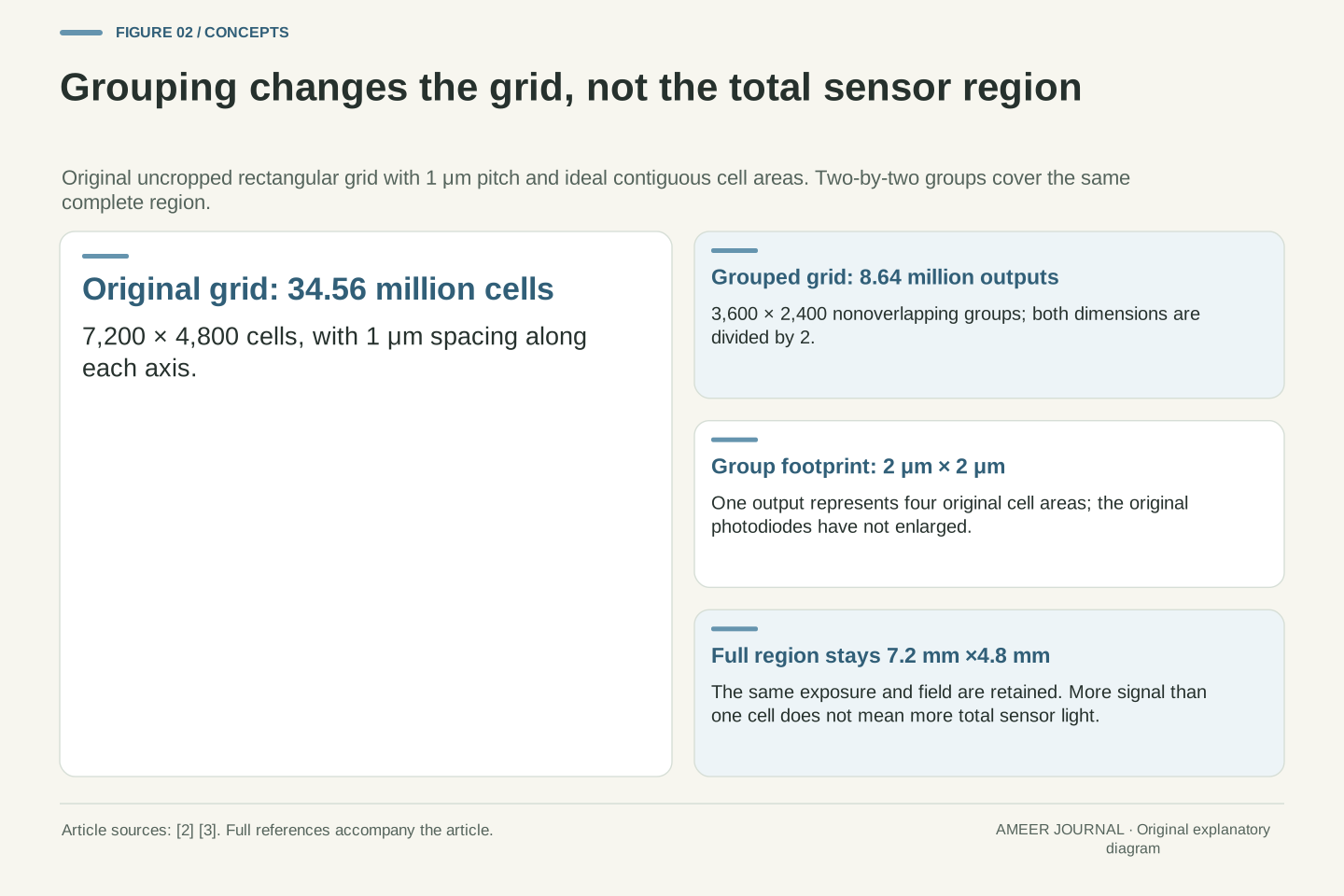
Imagine an ideal rectangular grid containing 7,200 cells across and 4,800 down. That is 34.56 million cells. Grouping them in nonoverlapping two-by-two squares gives 3,600 groups across and 2,400 down: 8.64 million outputs. The output count falls by four because both dimensions are divided by two. Basler's documentation likewise separates the horizontal and vertical grouping factors and describes the reduction in output dimensions. [2] Our dimensions are assigned for this example, not taken from a particular phone specification.

Give the original grid a one-micrometre spacing in each direction. Each group now spans two micrometres by two micrometres, covering four original cell areas. The complete represented region remains 7.2 millimetres by 4.8 millimetres. No new sensor area has appeared, and grouping the measurements does not collect a second exposure. A group contains more signal than one of its smaller cells when illumination is uniform because it includes four cells. Comparing that group with the original four-cell total is a different question from comparing it with one cell alone.

For the assigned W=7,200 and H=4,800 rectangular grid, WH=34,560,000 cells. Nonoverlapping 2×2 aggregation produces (W/2)(H/2)=8,640,000 outputs, with dimensions 3,600×2,400. The reduction is a factor of four in sample count and two along each axis. Basler documents separate binning factors and reduced effective output dimensions. [2] This example assumes an exactly divisible, uncropped grid; it does not infer an actual camera's active margins, processing crop or supported output size from its nominal sensor count.

Assign a 1 μm grid pitch and ideal contiguous square cell areas. The aggregate footprint is 2 μm×2 μm, while the total represented rectangle remains 7.2 mm×4.8 mm. Original photodiodes have not physically increased in size; the output measurement has broader spatial support. Holding that entire region and the exposure fixed prevents a fourfold group signal from being misreported as four times more photons collected by the whole sensor. The relevant baseline must state whether it contains one original cell or the same four-cell region.

The four-cell arithmetic below uses a monochrome measurement, or cells with the same spectral response. That condition is deliberate. A red-filter measurement and a blue-filter measurement do not describe identical slices of incoming light. Simply adding neighboring values with different meanings is not automatically the same operation as combining four matching measurements. Basler explicitly describes its colour-camera binning in terms of samples of the same colour. [2] A diagram that ignores those filter roles can make a clean-looking calculation describe the wrong operation.

The processing stage can change the meaning of the values too. Basler documents particular camera models that combine separate red, green and blue image planes after debayering. [2] That is different from a diagram showing four raw charge packets joined before readout. Samsung's phone-sensor grouping description does not settle which of our two noise models describes an arbitrary phone setting. [1] Keep the colour grouping and the combination stage as separate questions. Our four identical cells remove that complication so the later noise comparison has a clear, shared starting point.

Aggregation requires commensurate samples: their units and spectral response must support the intended scalar sum. The following model therefore stipulates monochrome cells, or an equivalent matched-response group. Basler's colour-camera description combines samples of the same colour. [2] It is not permission to treat every adjacent raw value as an independent measurement of the same band. A mixed-filter neighborhood would require an explicit colour-processing account before its sum could be compared with our monochrome signal and variance. Spatial adjacency alone does not establish that equivalence.

Basler also describes named models whose FPGA binning occurs after debayering, separately on the R, G and B planes. [2] That example establishes that the word binning can refer to a different data stage; it does not describe a phone's charge-domain operation. Samsung's documented binning/remosaic choices supply phone context without specifying the electrical assumptions used here. [1] The model consequently keeps filter meaning, aggregation stage and output normalization explicit. It neither reconstructs a colour-filter array nor evaluates the quality of a demosaicing or remosaic algorithm.

For the main example, suppose each equally illuminated cell detects an average of sixteen photoelectrons during one exposure. A particular exposure need not contain exactly sixteen. Hamamatsu explains photon-count fluctuations using Poisson statistics and separately identifies noise introduced when charge is read and converted into a value. [4][5] Assign each readout a noise spread of four electrons. Both numbers are invented inputs. The read error has zero average in this model, and the light fluctuations and read errors are independent across the four cells.

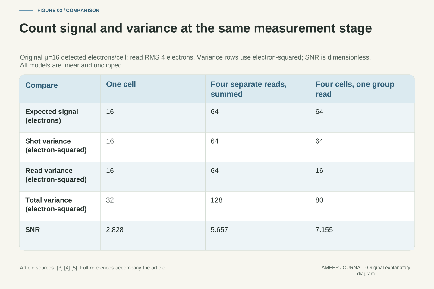
Noise spread is measured by its standard deviation. To combine independent contributions, square their spreads, add those variances, and take the square root. [5] A Poisson count with mean sixteen has variance sixteen and a spread of four electrons. Our read term adds another variance of sixteen, giving total variance thirty-two and a spread of about 5.66 electrons for one cell. Its signal-to-noise ratio is sixteen divided by 5.66, about 2.83. Background light, dark current, unequal response, clipping and rounding are excluded from this initial linear account.

Let X_i be independent Poisson detected-electron counts with mean μ=16. After offset removal and conversion to electron-equivalent units, define a separately read sample Y_i=X_i+R_i, where each R_i has zero mean and variance r²=16 for RMS read error r=4 electrons. Read errors are independent of one another and of all X_i. Hamamatsu's count-statistics and quadrature explanations support these distinctions. [4][5] Our μ counts detected electrons; it is not the incident-photon variable used in the source's quantum-efficiency formula.

Thus E[Y_i]=μ and Var(Y_i)=μ+r²=32 in electron-squared units. The standard deviation is √32≈5.657 electrons and the single-cell SNR is μ/√(μ+r²)=16/√32≈2.828. Squaring an RMS read noise changes its units: 4 electrons contributes 16 electron-squared to variance, not 16 electrons to standard deviation. The main model excludes background and dark terms, gain multiplication, quantization, saturation and response differences. Those exclusions define the calculation; they do not claim that real phone measurements lack those effects.

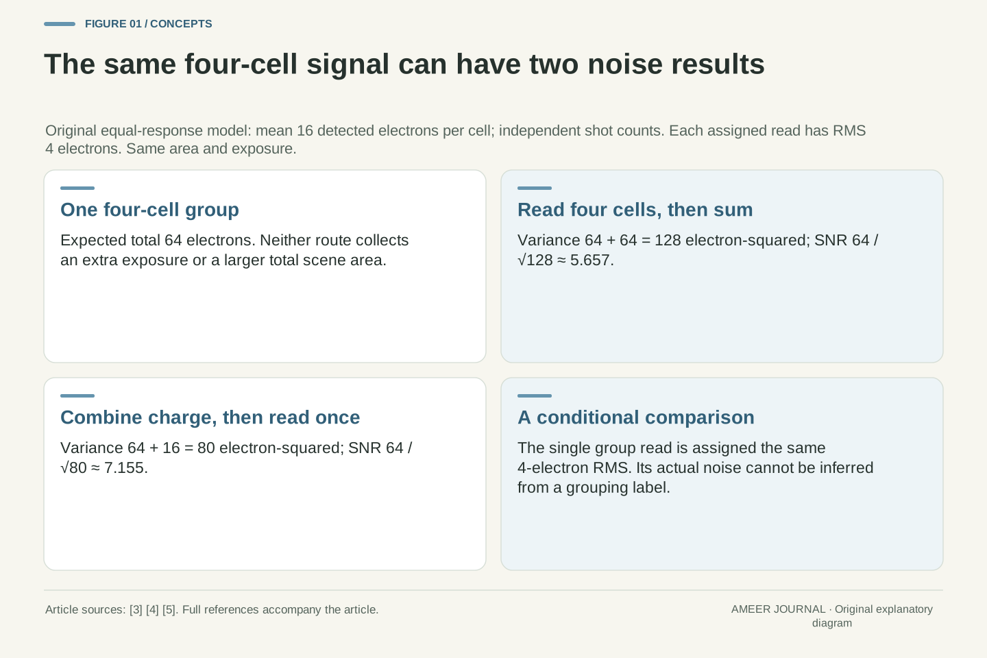
Read the four cells separately, then add their values. Their expected signal becomes sixty-four electrons. Because the four complete measurement errors are independent, their variances add to four times thirty-two, or 128 electron-squared. The total noise spread is the square root of 128, about 11.31 electrons. Dividing sixty-four by 11.31 gives an SNR of about 5.66. That is twice the single-cell SNR, although the expected signal is four times as large. The larger measurement covers four original cell areas, so this improvement does not come from an unchanged one-cell observation.

Now divide the entire sum by four to report an average instead. The expected value becomes sixteen, while the noise spread becomes 11.31 divided by four, about 2.83. Their ratio remains 5.66. Sum and average modes are documented options in Basler's binning description. [2] Within our exact, unclipped arithmetic, they differ only by a known scale factor. The sum may look brighter if displayed with unchanged settings, but a larger displayed number alone is not a higher SNR. Rounding or clipping would require an additional account beyond this simple rescaling.

For Z_d=ΣY_i across n=4 independent cells, E[Z_d]=nμ=64 and Var(Z_d)=n(μ+r²)=128 electron-squared. Its SNR is nμ/√[n(μ+r²)]≈5.657. Relative to one cell, the SNR gain is √n=2, while the signal gain is n=4. This comparison changes spatial support from one cell to four; the same-area comparison with another four-cell route follows next. Independent variances, rather than independent standard deviations, are the quantities being added. The four read operations contribute 64 electron-squared alongside 64 from shot fluctuations.

For the average A_d=Z_d/4, the mean is 16 and variance is 128/16=8 electron-squared. Its standard deviation is √8≈2.828, so SNR remains 16/√8≈5.657. Basler documents sum and average choices. [2] The present result is a linear-normalization identity: multiplying signal and noise by the same nonzero positive factor leaves their ratio unchanged. It does not establish identical clipping, output precision or processing in a real implementation. Likewise, summing these same four already-read samples later in software gives the same mathematical result, provided the values and operations remain unchanged.

Keep the same four cells, exposure and expected total of sixty-four photoelectrons. In the second route, combine their charge first, then measure that group once. Assign that one read the same four-electron noise spread as each earlier read. Hamamatsu's documentation describes pre-read combination in its CCD model and addition after digitization in its sCMOS simulation. [3] These are examples of different stages, not a rule that identifies every phone sensor. The equal four-electron read noise in our two routes is an explicit comparison assumption.

The light signal still fluctuates. Its four count variances add to sixty-four, and the single read contributes sixteen more, giving total variance eighty. The noise spread is about 8.94 electrons, so sixty-four divided by 8.94 gives an SNR of about 7.16. That exceeds the separately read sum's 5.66 for this same area. It is about 1.26 times that result, not four times. The advantage comes from replacing four assigned read-noise contributions with one. It does not remove shot noise, create extra light or prove that a real aggregation stage retains the same read noise.

Define Z_p=ΣX_i+R_g, where the four independent X_i retain μ=16 and the one group-read error R_g is independent with zero mean and variance r²=16. This represents charge aggregation before a single assigned read event. The documented simulator distinguishes pre-amplification/digitization CCD grouping from its modeled post-digitization sCMOS sum. [3] We adopt the stage distinction without asserting a universal sensor taxonomy. In particular, equal group-read and per-cell read RMS is stipulated, not deduced from the word analogue or from a megapixel setting.

The grouped mean is 64 and variance is nμ+r²=64+16=80 electron-squared. SNR is 64/√80≈7.155, versus 64/√128≈5.657 for separate reads. Their same-area ratio is √(128/80)=√1.6≈1.265. Relative to the smaller single cell, the pre-read result is about 2.530 times the SNR, which answers a different area comparison. The shot-noise variance has increased from 16 to 64 as four cells were included; only the count of stipulated read terms changed. A changed amplifier, transfer noise or saturation behavior would require a different model.

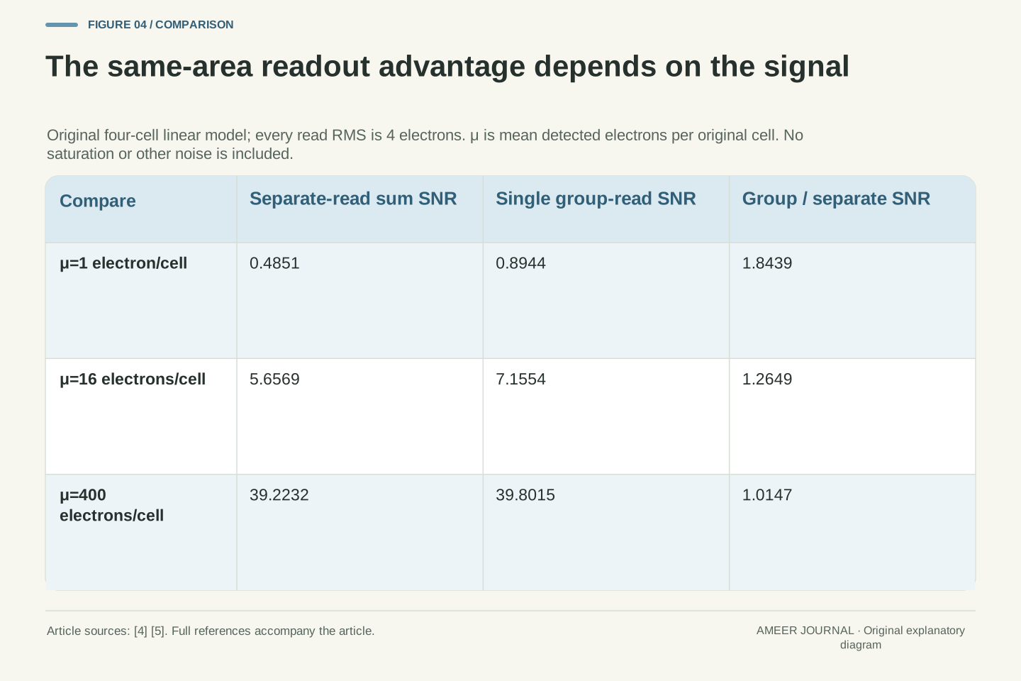
Repeat the same four-cell comparison with a mean of only one detected electron per cell. Keep every assigned read-noise spread at four electrons. The separately read sum has an SNR of about 0.485, while the pre-read group has about 0.894. The latter is roughly 1.84 times the former. Neither value is a phone measurement or a judgment about a finished photograph. This low-signal example simply makes the extra read contributions large beside the small expected group signal of four electrons.

Now use a separate mean of four hundred electrons per cell, retaining the unclipped linear assumptions. The two SNRs become about 39.22 and 39.80, much closer together. Signal-dependent shot fluctuations now dominate more of the variance, so removing three read terms changes less. Hamamatsu distinguishes shot noise from the read component. [4][5] Our exact ratio approaches one as signal becomes very large in this mathematical model. A fixed four-cell grouping therefore cannot establish one improvement factor for every illumination level, even before real processing or hardware differences enter the comparison.

For arbitrary positive μ with n=4 and r=4, the separate-read SNR is 4μ/√(4μ+64), while the pre-read SNR is 4μ/√(4μ+16). Their ratio is √[(μ+16)/(μ+4)]. At μ=1, these give approximately 0.4851 and 0.8944, with ratio √(17/5)≈1.8439. At μ=400, they give approximately 39.2232 and 39.8015, with ratio √(104/101)≈1.01474. These are independent assigned illumination cases; they do not identify a real sensor's operating range or imply that an actual device remains unsaturated.

The squared ratio equals 1+12/(μ+4), so it decreases as positive μ increases. It approaches four as μ approaches zero from above, making the SNR ratio approach two; at exactly zero signal, dividing the two zero SNRs would be undefined. At large μ, the ratio approaches one. The shot/read distinction is documented, while these limits follow from our equations. [4][5] They concern the same four-cell area, not the different comparison against one original cell, and do not establish an overall image-quality or dynamic-range multiplier.

The earlier sums depend on independent read errors. Change that assumption in a separate example: suppose one fluctuating error is added equally to all four measurements during an exposure. Its average is zero and its noise spread is four electrons. Each individual cell still has the same sixteen-electron expected signal and total variance of thirty-two as before. Yet the errors now move together. If the shared error is positive in one exposure, every cell carries that same positive contribution instead of four independent contributions that can partly balance.

When the four values are added, that shared error is multiplied by four. Its variance becomes 256 electron-squared, not sixty-four. Add the independent shot variance of sixty-four and the group variance becomes 320, giving an SNR of about 3.58. The earlier independent-read sum gave 5.66 with identical individual-cell variances. Hamamatsu's quadrature rule explicitly concerns uncorrelated noise. [5] This constructed counterexample explains why that condition matters. It does not claim that a particular phone has this fully shared error; it shows what a single per-pixel noise figure leaves unresolved.

Define a separate model Y_i=X_i+Z, with the independent Poisson X_i still having μ=16, and one common random Z independent of all counts, with E[Z]=0 and Var(Z)=16. Each marginal Var(Y_i)=32 matches the earlier model. However, Cov(Y_i,Y_j)=16 for distinct cells because their read contribution is shared. Summing marginal variances alone would therefore omit covariance terms. The source's quadrature statement is specifically qualified by uncorrelated noise. [5] No observed sensor covariance is being estimated here; Z is an assigned analytical construction.

For the group, ΣY_i=ΣX_i+4Z. Its mean remains 64, but variance is 64+16×16=320 electron-squared. Equivalently, four marginal variances contribute 128 and twelve ordered cross-covariance terms contribute 192. SNR is 64/√320≈3.578, and the averaged output has variance 320/16=20. Thus equal per-cell SNRs do not determine equal aggregate SNRs. The independent and shared-error models have the same single-cell moments but different joint behavior. A real comparison would need evidence about those relationships rather than assuming that a published noise number settles them.

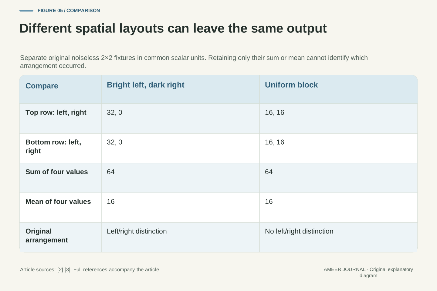
Set noise aside for a separate, exact four-value picture. One two-by-two block has top row thirty-two, zero and bottom row thirty-two, zero: its left side is brighter than its right. Another block contains sixteen in every position. Both blocks sum to sixty-four and average to sixteen. After keeping only that sum or mean, the output does not tell us which arrangement occurred. Combining samples has removed a spatial distinction even though it preserved the total of their assigned values.

There are six ways to place two bright values of thirty-two among four positions, and every one gives the same total of sixty-four. The uniform block gives that total too. No reversal of the scale from sum to average can separate them afterward. Binning's tradeoff with spatial sampling is documented. [2][3] Additional exposures, neighboring measurements or a reconstruction prior could supply extra information, but that information is not contained in the single number alone. A less noisy aggregate and a more informative map of positions are therefore different properties to examine.

Consider two deterministic, noiseless input vectors ordered by rows: a=(32, 0, 32, 0) and b=(16, 16, 16, 16). The sum operator L(x)=x_1+x_2+x_3+x_4 gives L(a)=L(b)=64 although a≠b. Averaging merely applies L/4, yielding 16 for both. The aggregation is therefore non-injective: it maps distinct spatial inputs to the same output. This is an exact finite example of discarded within-group information, consistent with the documented sampling tradeoff. [2][3] It is separate from the earlier uniform Poisson-noise constructions and does not represent a photographed target.

Restricting inputs to zero or 32 with exactly two bright positions already supplies six distinct arrangements, since there are six choices of two positions among four. Their scalar sums coincide. Recovering which arrangement occurred requires additional information or assumptions; rescaling the retained scalar cannot provide that identification. This statement does not deny reconstruction from other frames or scene structure. It isolates what the chosen output retains. An SNR gain for that aggregate consequently does not establish preserved edge position, greater optical resolving power or a fourfold improvement in spatial detail.

The linear noise examples have not assigned a saturation limit. That is a separate input. Hamamatsu defines full-well capacity as the maximum charge a pixel can accumulate before saturation and distinguishes it from output bit depth. [3] A group containing four cells does not, from that fact alone, tell us the capacity of a later stage that combines or represents their signals. Likewise, a large output value may be a scaling choice rather than evidence that more usable charge can be recorded. The ceiling needs its own specification.

Use a separate deterministic fixture: four individual wells can each hold one hundred electrons and currently contain exactly ninety each. Their total is 360. Assign the following grouping node a limit of 250 electrons and stipulate that it clips there. Although no individual well has reached its own limit, the combined stage cannot represent the remaining 110 electrons. This is a new illustrative capacity model, not a limit imposed on the earlier noise examples or a real phone circuit. A noise benefit alone therefore cannot establish how much bright signal remains distinguishable before saturation.

The preceding SNR formulas describe an unclipped linear measurement. Full-well capacity, later-stage signal capacity and output numerical range require additional constraints. Hamamatsu separately defines full well and bit depth, while Basler warns that sum normalization can increase the apparent response to light. [2][3] Neither statement provides the capacities of our hypothetical aggregator. A count of four input cells cannot establish that every downstream stage accepts four times one cell's maximum charge, nor that a derived reduction in noise automatically becomes a proportional increase in usable dynamic range.

In a separate deterministic construction, let each input well permit 100 electrons and hold 90, while a combined node represents min(Q, 250) electrons for total charge Q. Then Q=4×90=360 and the node represents 250; 110 electrons of that input total lie beyond its assigned representable capacity. These are exact supplied charge packets, not Poisson means being substituted into a clipping function. The earlier μ=400 noise case belongs to the separate unclipped model. Real overflow, transfer and conversion behavior would need its own description; this fixture only disproves inference of the aggregate ceiling from the number of input wells.

Suppose a saved high-resolution measurement retains the same four separately read values used in our first route. Adding those values later produces exactly the same sum; averaging them later produces the same average. The arithmetic has not acquired an extra readout advantage merely because it runs inside a camera. Hamamatsu makes this comparison within its stated post-digitization sCMOS simulation. [3] A claim of an additional benefit must identify something that changed before or during those measurements, or another processing step beyond the defined linear operation.

For an actual comparison, keep the scene area, exposure and displayed scale visible. One large group and one smaller native pixel cover different areas, even if both occupy one square on a screen. Different phone modes can also present different processing and representations, as Samsung's binning/remosaic description illustrates. [1] Our equations do not rank those finished outputs. They provide questions to ask: were the same measurements combined, were read errors already present, and did the comparison preserve spatial support? Those questions are more informative than treating a lower megapixel count as a complete noise specification.

For retained separately read samples Y_i, an offline implementation of ΣY_i is algebraically identical to the defined digital aggregation route. Division by four produces the same normalized average if neither implementation adds rounding, clipping or other transformations. Hamamatsu's simulator documentation explicitly distinguishes that post-digitization equivalence from its modeled pre-read charge combination. [3] The equivalence does not cover different raw measurements, exposures, sensor modes or nonlinear processing. It identifies the restricted case in which moving the same arithmetic to another location cannot change its statistical result.

A controlled comparison therefore names the represented scene area, exposure, spectral response, sample stage, numerical scaling and output support. One-cell versus four-cell comparisons and two same-area four-cell routes answer different questions. Samsung's phone-mode descriptions establish representation choices, not the equality of all those experimental conditions. [1] Nor does equal output size prove equal retained detail, as the two spatial patterns showed. The resulting SNR is conditional on a specific measurement model; determining a real phone's behavior would require documentation or measurements that identify its actual acquisition and processing path.

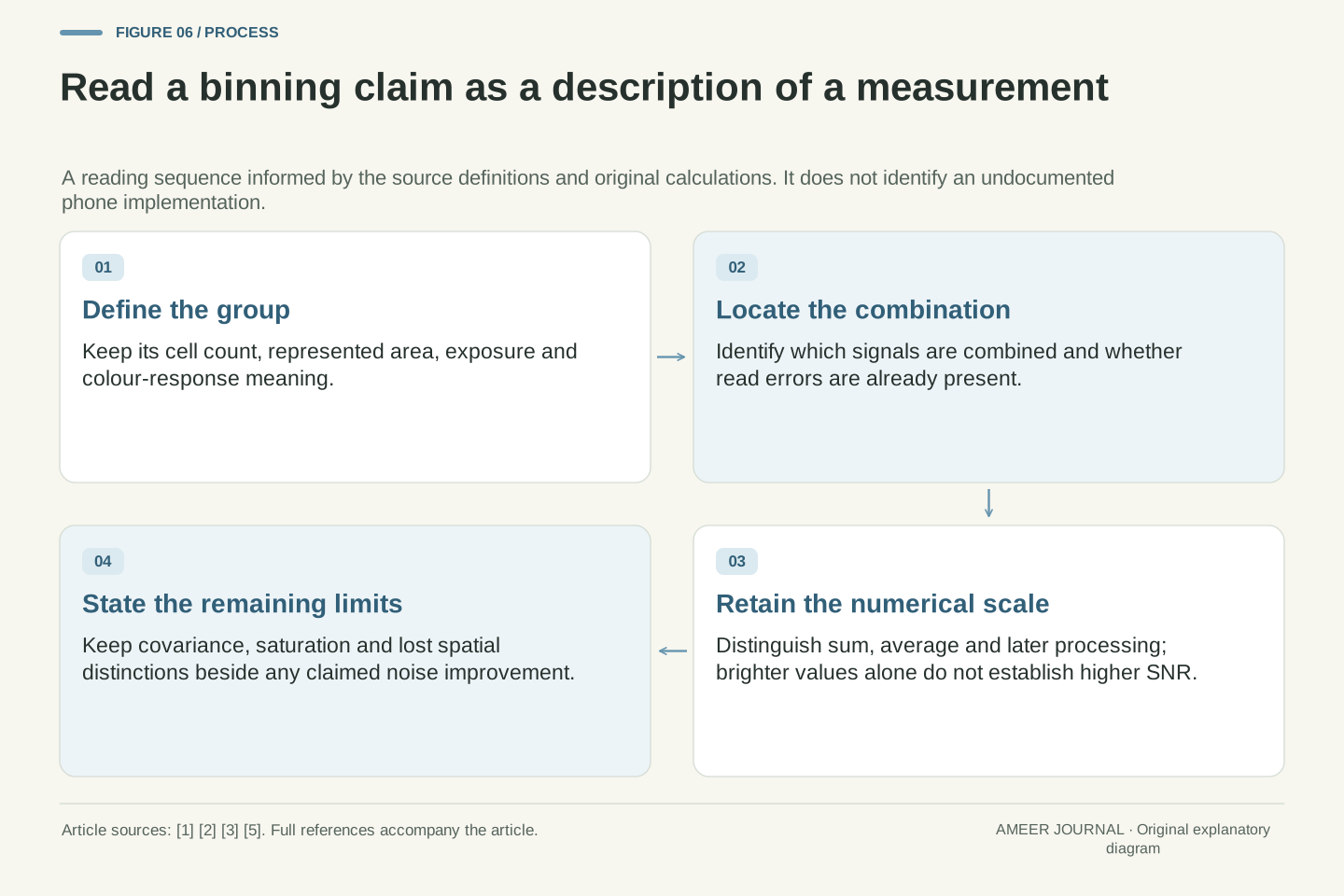
A useful description of binning starts with the group: how many cells contribute, what area they cover and whether their colour responses match. It then states when they are combined and whether the result is a sum, an average or something more elaborate. The documented sensor, FPGA and simulated charge-versus-digital examples show why these are separate questions. [2][3] Finally, it names the noise assumptions and signal limits. Without those details, the grouping factor remains a partial description rather than a complete explanation of the output.

Our four-cell group had a mean signal of sixty-four in both readout routes, yet its SNR was about 5.66 after four separate reads and 7.16 after the assigned single group read. A shared-error construction changed the result again, while different spatial patterns still produced the same scalar output. None of those distinctions is visible in the phrase four-to-one alone. Read the smaller image dimensions as a starting fact, then ask which measurements and transformations produced them. That keeps numerical brightness, noise quality and retained spatial information from being mistaken for the same improvement.

Retain six items: group geometry, spectral meaning, aggregation stage, normalization, noise covariance and signal capacity. Source documentation supplies examples of these distinctions, while the calculations show why they cannot be collapsed into one multiplier. [1][2][3][5] The independent-read model, pre-read model and common-error model use related marginal quantities but yield different aggregate variances. The deterministic spatial and saturation fixtures impose different information limits again. Each conclusion belongs to the model whose assumptions produced it; no undocumented phone feature is needed to establish the mathematical distinction.

The central result is conditional and useful: grouping four equal-response cells increases the represented area relative to one cell, but a same-area noise comparison depends on the read terms and their correlations. Sum versus average is only a scale change in exact linear arithmetic. Spatial aggregation can discard arrangements even when its aggregate SNR improves, and maximum representable signal requires separate evidence. A phone's binning label can help locate those questions, but it cannot answer them all without the accompanying acquisition and processing description.