What you’ll take away
- The Switch-style balancing score combines hard assignment fractions f with mean router probabilities P; neither summary can be recovered from the scalar alone.
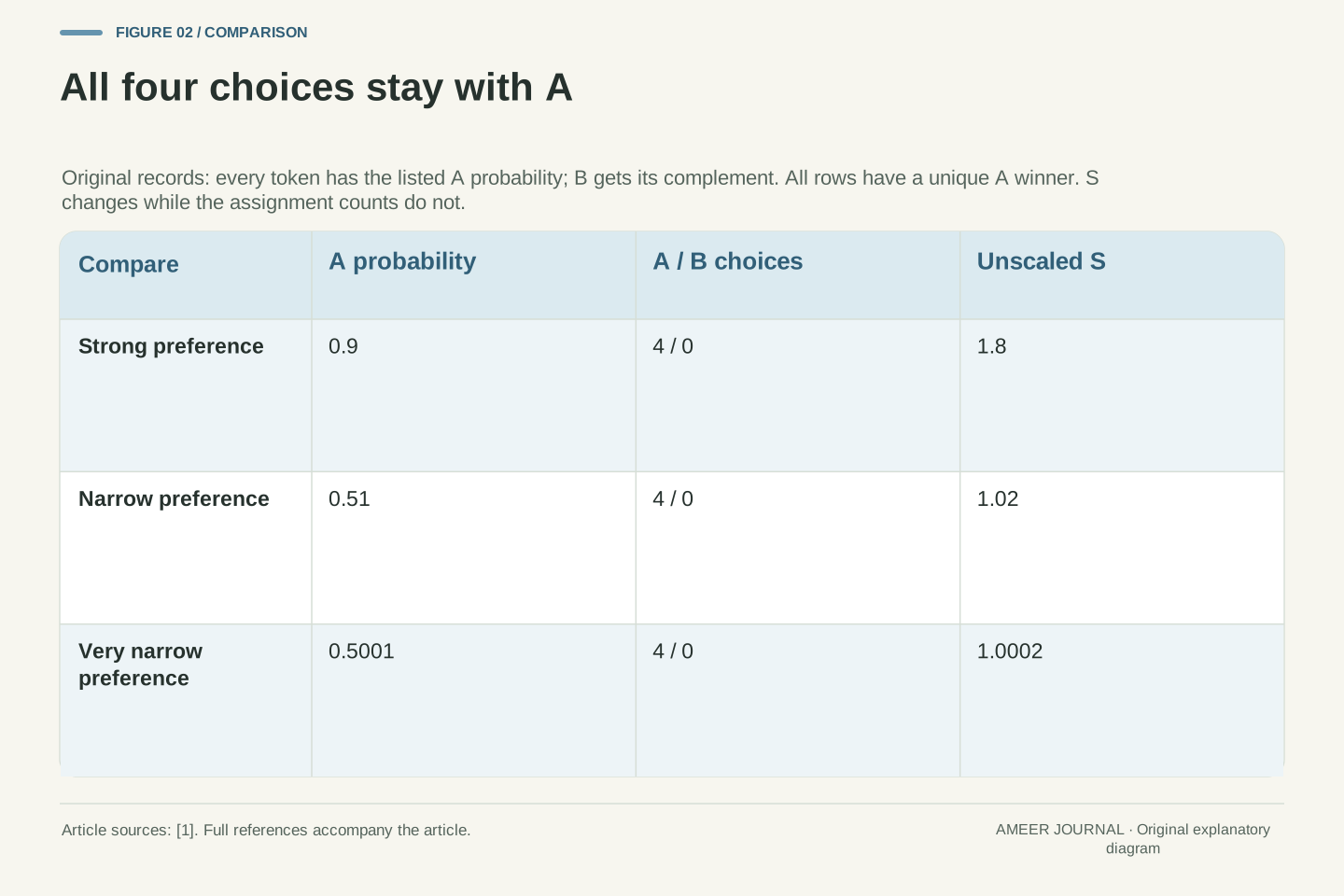
- The same four-to-zero choices give S values of 1.8, 1.02 and 1.0002 as the winning probability changes.
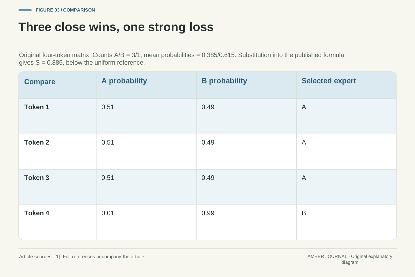
- An explicit three-to-one assignment record gives S=0.885, so the uniform reference of one is not a universal finite-record lower bound.
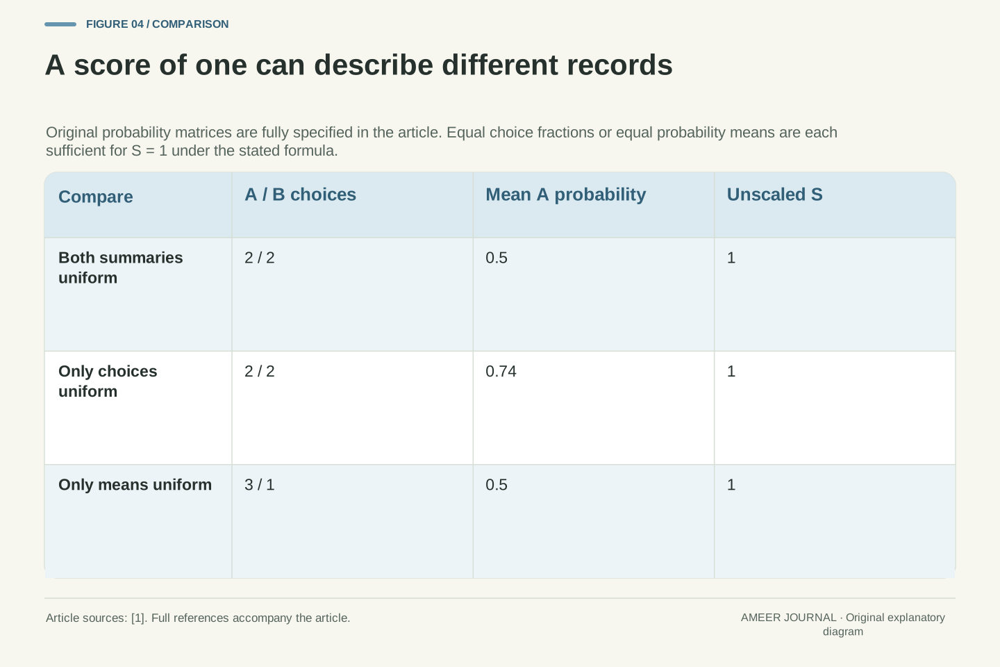
- Uniform assignment fractions or uniform probability means each give S=1 under the stated normalization.
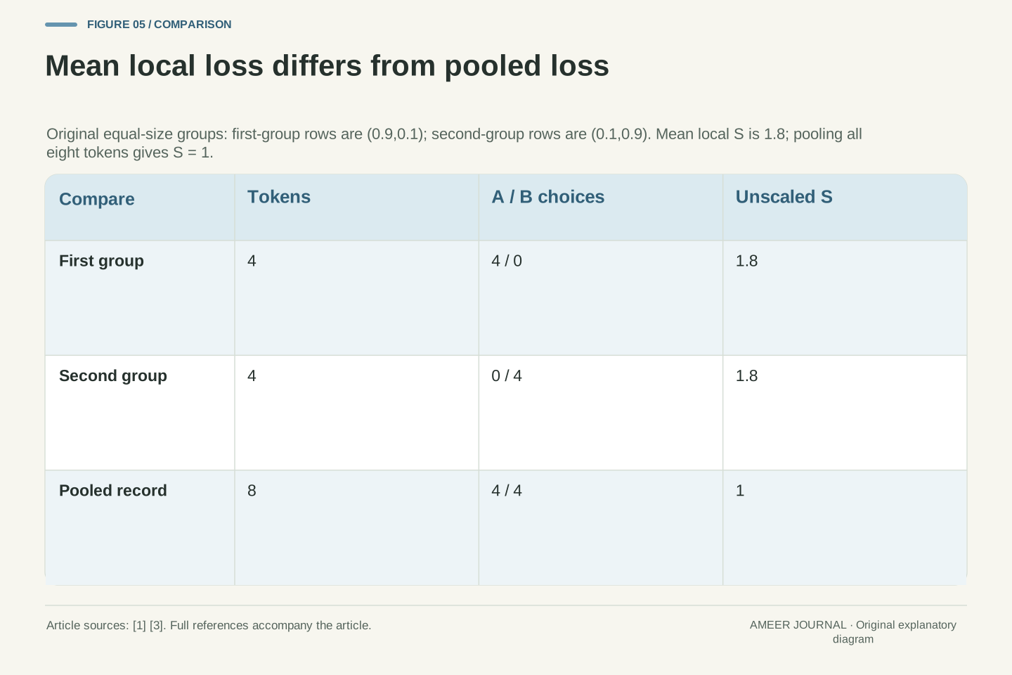
- Two opposite one-sided groups can each score 1.8 while their combined record scores 1; grouping is part of the statistic.
- Keep token counts, probability means, coefficients, routing stage and aggregation rules alongside the logged loss.
What does the router’s balancing score measure?
An AI model with several expert networks needs a rule for choosing which expert receives each token. A router can assign a score to every available expert, then choose the highest. During training, an extra loss can encourage work to spread across experts. The Switch Transformer paper describes one such loss [1]. But reading that loss is different from counting where the work went.
Suppose a dashboard shows the balancing loss getting smaller. Did an overloaded expert receive fewer tokens, or did the router simply become less confident about sending the same tokens there? Both possibilities deserve attention. The number combines the actual choices with the probabilities behind those choices. It does not display either set of information separately.
We will use invented records containing four tokens and two experts, called A and B. Each token chooses exactly one expert. There are no tied scores, padding tokens or rejected assignments. These are arithmetic examples, not measurements from a trained model. Keeping the records small lets us inspect every choice and understand precisely what the loss can tell us.
A Switch-style auxiliary balancing loss combines a hard assignment distribution with a mean router-probability distribution. It is a training objective, not a direct encoding of the expert-load histogram. Equations 4–6 of the pinned Switch Transformer manuscript supply the definition used here [1]. Our examples examine the information retained and lost by that scalar.
Scope is one top-one routing layer with N experts and T valid tokens. Each token has a strictly positive normalized probability vector and a unique argmax. We assume no capacity drops, padding or additional routing restrictions. The probability matrices, scalar comparisons and gradient calculations are constructed examples; no model training, deployment or implementation benchmark is claimed.
This restriction matters because a general MoE system may select several experts or normalize assignment counts differently. NVIDIA’s named balancing-loss function explicitly includes topk in its count denominator [3]. Here topk equals one throughout. We do not transfer conclusions about the exact numerical scale to every router merely because its log contains a similarly named auxiliary-loss field.
Count the choices, then average the probabilities
For each token, write two probabilities that add to one. The larger probability determines the selected expert. If the pair is 0.51 for A and 0.49 for B, the token chooses A in our rule. That is one complete choice for A, not half a token for each expert. The probabilities describe the router’s scores before the choice [1].
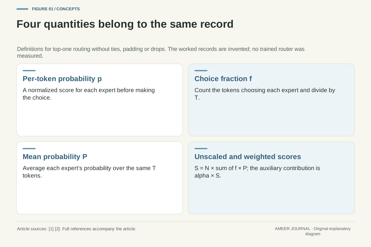
Now make two summaries. First, count the tokens choosing each expert and divide by the total number of tokens. We call these choice fractions f. Second, average each expert’s probabilities across all tokens. We call these averages P. With four tokens, one additional choice changes a choice fraction by one quarter, while the average probability can change by a much smaller amount.
For a first record, let A’s probabilities be 0.8, 0.7, 0.3 and 0.2; B gets the remainder in each row. Two tokens choose each expert. Both choice fractions are 0.5, and both average probabilities are also 0.5. This convenient starting record has equal choices and equal average scores. Later records will separate those properties.
Let p_ti be the probability for expert i on token t, with sum_i p_ti=1. Define f_i=(1/T) sum_t 1{argmax_j p_tj=i} and P_i=(1/T) sum_t p_ti. These are the hard assignment fraction and mean probability respectively [1]. Both sum to one under our assumptions, but they are generally different vectors.
For N=2 and T=4, use A probabilities (0.8,0.7,0.3,0.2), with B probabilities their complements. The assignment counts are (2,2), so f=(0.5,0.5). Summing A’s probabilities gives 2, hence P_A=0.5 and P_B=0.5. This example intentionally makes both distributions uniform; that coincidence is not part of their definition.
The hard fractions have increments of 1/T, whereas the probability means vary continuously within a region of unchanged argmax decisions. A strictly positive normalized row is compatible with a softmax: choosing logits equal to the logarithms of its probabilities reproduces that row. Our later matrices therefore do not require impossible probability values to demonstrate the distinction. They do not claim that a particular trained network produced those logits.
Separate the unscaled score from its weight
Multiply each expert’s choice fraction by its average probability, add the results, and multiply by the number of experts. Call this unscaled score S. For our starting record, S is 2 times the sum of 0.5 times 0.5 and 0.5 times 0.5. The result is 1. The original paper then multiplies this score by a coefficient called alpha before adding the auxiliary term to the training loss [1].
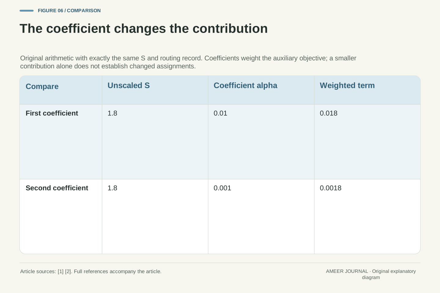
The coefficient changes how strongly this term is weighted. If S is 1.8, multiplying by 0.01 gives 0.018. Multiplying the same S by 0.001 gives 0.0018. The second reported contribution is ten times smaller even though every probability and every expert choice is unchanged.
This is why a log needs to say which number it reports. The historical paper uses 0.01, while the pinned Transformers 4.49.0 configuration documents an auxiliary coefficient default of 0.001 [1][2]. Those are facts about those sources, not a recommendation to copy either value. Comparing two runs requires their actual coefficients and logging definitions.
Write S=N sum_i f_i P_i and L_aux=alpha S. This separates the unscaled quantity from the weighted contribution in the original formula [1]. At the uniform reference f_i=P_i=1/N, the dot product is 1/N and S=1. Multiplication by N keeps that reference value independent of the expert count.
For S=1.8, alpha=0.01 yields L_aux=0.018, whereas alpha=0.001 yields 0.0018. The routing statistics are identical. A lower weighted term cannot establish improved allocation unless the coefficient and other reductions are held comparable. The total task objective may contain additional terms, so its magnitude cannot be read as S either.
The manuscript reports alpha=0.01 for its experiments. Transformers v4.49.0 documents router_aux_loss_coef=0.001, separately from router_z_loss_coef [1][2]. This versioned difference illustrates why coefficients belong in a reproducibility record. It neither compares the quality of those systems nor establishes a current default for another release, model configuration or training recipe.
A score of one does not uniquely identify a state
The starting example gives S equal to 1. Now change A’s probabilities to 0.99, 0.99, 0.49 and 0.49. The first two tokens still choose A, and the last two choose B. Choices remain evenly split, but A’s average probability becomes 0.74 and B’s becomes 0.26. The score is still 1: 2 times the sum of 0.5 times 0.74 and 0.5 times 0.26.
In fact, whenever the choice fractions are equal, this formula gives S equal to 1 regardless of how the average probabilities are divided. Equal choices are enough to produce the reference value. They are not enough to prove that the router’s average scores are equal too.
The reverse implication also needs care. A value of 1 does not prove that the choices were evenly split. We will build that counterexample shortly. Treat 1 as a useful reference calculation, not a certificate describing every part of the router. A single output number cannot show the full pair of distributions that produced it.
If f_i=1/N for every i, then S=N sum_i (1/N)P_i=sum_i P_i=1. Uniform hard assignments therefore give S=1 for any normalized P. This algebraic property is stronger than checking only the joint-uniform reference, and it shows why S cannot certify uniformity of both vectors.
For A probabilities (0.99,0.99,0.49,0.49), f=(0.5,0.5) but P=(0.74,0.26). The scalar remains 1. The equal assignment counts do not imply equal mean confidence, and the unchanged scalar does not reveal the confidence shift from the first example. Both matrices have unique argmax decisions and positive entries.
The original paper motivates the objective through balanced routing [1]. Here we distinguish that training motivation from finite-batch identifiability. Observing S=1 does not uniquely recover f or P, and the reference calculation by itself is not a proof that 1 is a universal lower bound over every admissible finite probability matrix. The next examples make both limitations explicit.
The loss can fall while all four choices stay put
Give all four tokens the same probabilities: 0.9 for A and 0.1 for B. Every token chooses A. The choice fractions are 1 and 0, and the average probabilities are 0.9 and 0.1. The unscaled score is therefore 1.8. Nothing in this record is evenly divided between the experts.
Reduce A’s probability to 0.51 for every token and raise B’s to 0.49. A still wins every choice, but S falls to 1.02. Make the pair 0.5001 and 0.4999, and S becomes 1.0002. The score is now very close to the uniform reference even though B still receives no tokens at all.
The reason is that our router chooses the larger probability; it does not randomly divide tokens according to those probabilities. A narrow winning margin is still a win. The example separates a useful change in confidence from a change in assignment counts. A dashboard showing only the loss cannot tell you which change happened.
For four identical rows (q,1−q) with q>0.5, every token selects A. Thus f=(1,0), P=(q,1−q) and S=2q. Choosing q=0.9, 0.51 and 0.5001 gives S=1.8, 1.02 and 1.0002 respectively, while the histogram stays (4,0).
As q approaches 0.5 from above, S approaches 1 without any change to the hard assignment fractions. We exclude the exact tie, so no tie-breaking convention is needed. This is an explicit sequence of valid matrices whose scalar approaches the uniform reference while one expert receives every attempted assignment.
The interpretation depends on deterministic argmax selection, as declared. It is not a claim about a router that samples experts from p, applies additional balancing constraints or uses another objective. Within the stated rule, decreasing confidence can lower S before any argmax changes. The loss and the assignment histogram answer different questions even when calculated from the same tokens.
An uneven record can even score below one
Consider a different four-token record. The first three tokens each give A probability 0.51 and B probability 0.49. The fourth gives A probability 0.01 and B probability 0.99. Three tokens choose A and one chooses B, so the choice fractions are 0.75 and 0.25.
Average the scores separately. A’s total is 0.51 plus 0.51 plus 0.51 plus 0.01, which is 1.54. Dividing by four gives 0.385. B’s average is 0.615. The unscaled score is 2 times the sum of 0.75 times 0.385 and 0.25 times 0.615. That gives 0.885, below the evenly split starting record’s score of 1.
There is no missing token or rounding trick. A wins three close contests, while B wins one very strongly. Those different margins pull the average probabilities toward B despite A winning more choices. This invented record shows why a lower scalar does not always rank two assignment histograms by how evenly they divide the work. It does not report a failed training run.
Set the first three rows to (0.51,0.49) and the fourth to (0.01,0.99). The unique argmax assignments yield f=(3/4,1/4). The probability means are P=(77/200,123/200)=(0.385,0.615). Hence S=2[(3/4)(77/200)+(1/4)(123/200)]=177/200=0.885.
The uniform-count reference has S=1, although its count split is (2,2) rather than (3,1). Thus the scalar does not monotonically rank these finite records by count equality. All row entries are positive and all row sums equal one. The construction uses the published algebra directly, without invoking capacity filtering, padding or numerical underflow.
The manuscript’s uniform-routing motivation and minimum wording [1] should therefore not be converted into an unconditional finite-batch assertion that S cannot fall below one. Our narrower conclusion follows from the explicit matrix: neither a small value nor comparison with the uniform reference certifies balanced hard counts. It does not establish the frequency of this situation in training or overturn an empirical result about model quality.
The score combines two kinds of imbalance
The previous record puts more choices on A but more average probability on B. The score mixes those two summaries through multiplication. It is not simply measuring how far the choice counts are from an even split. That distinction explains the apparently surprising value below 1.
For another example, give the first three tokens A probability 0.6 and the fourth A probability 0.2. A again wins three choices. Its average probability is now exactly 0.5, and B’s is also 0.5. The score returns to 1 despite the uneven 3-to-1 choice count.
Together the examples show three different meanings hidden behind a familiar value. A score of 1 can accompany equal choices and equal averages, equal choices and unequal averages, or unequal choices and equal averages. Keeping both summaries beside the scalar makes the record understandable. The extra information comes from retaining the inputs to the calculation, not from interpreting more digits of the final score.
Using sum_i f_i=sum_i P_i=1, expand the score as S=1+N sum_i(f_i−1/N)(P_i−1/N). The second term is a dot product of deviations from uniformity, not a squared distance of f from uniformity. Its sign depends on how the deviations of the two vectors align.
In the 0.885 example, those deviations are (0.25,−0.25) and (−0.115,0.115). Their dot product is negative. Conversely, if P is uniform, S=1 for any normalized f. The matrix with A probabilities (0.6,0.6,0.6,0.2) gives f=(0.75,0.25), P=(0.5,0.5) and exactly that result.
This decomposition explains the loss of identifiability without claiming that f and P can be chosen independently of a valid routing matrix. Each numerical case supplies the matrix that generates both. It also avoids treating S as a divergence of the hard-count distribution: the second vector is essential to its definition, and replacing it would define a different statistic.
A gradient can move probabilities before choices change
Why use a score involving probabilities at all? Small changes to a router’s scores can change its probabilities even when the winning expert stays the same. The paper distinguishes the probability part, through which the loss can be differentiated, from the hard choice fraction [1]. This supplies a direction for adjusting the router during training.
In the all-A record, lowering A’s probabilities while keeping them above B’s lowers the score without moving any token. Our earlier sequence from 0.9 to 0.51 demonstrates that effect directly. The loss is responding to something real in the invented record: the strength of the router’s preference. The unchanged histogram is also real.
Once a winning expert changes, the choice fractions must be counted again. A calculation describing tiny changes that keep every winner fixed cannot predict every later step of training. Other loss terms also affect a real update. Reading a local training signal as a complete promise about the next allocation would give it more meaning than the calculation supports.
Within a region where every argmax is unchanged, treat f as constant and let p_t be softmax(z_t). Differentiating S gives ∂S/∂z_tj=(N/T)p_tj[f_j−sum_i f_i p_ti]. This is our local derivation from the published formula [1], not execution of a library’s backward pass.
For N=2, T=4, f=(1,0) and each row (0.51,0.49), the derivatives for one token’s A and B logits are +0.12495 and −0.12495. Gradient descent on this term alone tends to reduce that token’s preference for A locally. The weighted term multiplies both derivatives by alpha. Our finite-difference checks preserve the original argmax assignments throughout.
If f is uniform, this local derivative is zero for any p_t because the bracket vanishes. At an argmax boundary the fixed-f derivation no longer describes the complete piecewise function; f must be recomputed. We make no guarantee about a finite optimizer step, parameter sharing across tokens, other objective terms or the eventual histogram of a trained network.
Combining groups changes the question
Imagine two groups of four tokens. Every token in the first group has probabilities 0.9 for A and 0.1 for B. Every token in the second has the reverse probabilities. Each group sends all its tokens to one expert. Calculating S separately gives 1.8 for each group, so their average score is 1.8.
Now combine the eight tokens before making the summaries. Four choose A and four choose B. The combined average probabilities are 0.5 and 0.5, and the combined score is 1. The probabilities and choices have not changed. We changed which records were grouped together for the calculation.
Both answers are correct for their stated grouping. The combined record is evenly split overall, while each smaller record is completely one-sided. A global number can therefore hide differences between its parts. These groups are invented collections of records; we are not claiming to measure a device, a distributed training system or the workload of a particular processor.
Let group A contain four rows (0.9,0.1) and group B four rows (0.1,0.9). Their local scores are both 1.8. Pooling the sufficient statistics gives f_pool=(0.5,0.5), P_pool=(0.5,0.5) and S_pool=1. The mean local objective and the objective evaluated on pooled means are different calculations.
For groups g with token weights w_g=T_g/sum_h T_h, define f_pool=sum_g w_g f_g and P_pool=sum_g w_g P_g. The weighted mean local score is N sum_i sum_g w_g f_gi P_gi. The pooled score is N sum_i(sum_g w_g f_gi)(sum_g w_g P_gi). Multiplying means generally differs from averaging products.
The equal opposite groups provide a concrete difference of 0.8 between those scores. This does not diagnose a distributed implementation. It establishes that the aggregation boundary is part of the statistic’s meaning. NVIDIA’s documentation likewise distinguishes batch levels and the matching count denominators [3]; its complete distributed procedure is outside this finite-record example.
Unequal groups need unequal weights
Change the example so that the first group has three tokens, each favouring A by 0.9 to 0.1. The second group has just one token, favouring B by 0.9 to 0.1. Each group still has an individual score of 1.8. Together, however, the choices are three for A and one for B.
The combined average probability for A is the sum of 0.9, 0.9, 0.9 and 0.1 divided by four: 0.7. B’s average is 0.3. With choice fractions 0.75 and 0.25, the combined score is 2 times the sum of 0.75 times 0.7 and 0.25 times 0.3, giving 1.2.
Giving the two groups equal weight would lose the fact that one contains three times as many tokens. Weight each group by its token count when rebuilding the combined summaries. Keep the choice counts and their denominator at the same level. That is also a specific requirement in NVIDIA’s documented balancing-loss arguments [3].
Take T_A=3 rows (0.9,0.1) and T_B=1 row (0.1,0.9). The token weights are 3/4 and 1/4. Thus f_pool=(0.75,0.25) and P_pool=(0.7,0.3), giving S_pool=2(0.75×0.7+0.25×0.3)=1.2. Each local score is still 1.8, so their token-weighted mean is also 1.8.
An unweighted average of the two local fractions would instead produce (0.5,0.5), which is not the pooled assignment fraction. The same error would affect the probability means. The denominator must refer to the population whose numerator is being summarized; matching array lengths or using two groups does not establish that consistency.
NVIDIA’s retrieved nightly documentation says tokens_per_expert should represent the intended batch level and total_num_tokens should match that level, while probs refers to the local batch being processed [3]. Our calculation demonstrates the count-and-denominator principle only. It does not replace the documented distributed reduction with a naive average of independently returned local values.
Keep the routing stage and other losses visible
There is another boundary to record: are we counting the experts initially selected, or the tokens those experts actually process? Our examples assume every selected token is processed. A router with a capacity limit may not satisfy that assumption. The pinned Transformers documentation explicitly warns that its router does not guarantee an expert processes every token [2].
The original paper’s pseudocode calculates its balancing term from the initial choice mask before later capacity filtering [1]. That ordering matters when interpreting the counts. A log of accepted work after filtering is not automatically the same input that was used for the auxiliary score. Keep the stage named instead of silently comparing different counts.
Also keep the balancing term separate from router z-loss. The pinned configuration gives them separate coefficients, and NVIDIA describes z-loss as encouraging smaller logits for stability [2][3]. A combined label such as router loss can hide that distinction. Neither term by itself supplies an answer about generated text quality, elapsed time or whether a particular expert learned a useful skill.
The finite records use attempted top-one assignments, with no filtering. The manuscript pseudocode constructs the argmax mask, computes auxiliary loss, and only then applies the capacity mask [1]. The pinned Hugging Face router documentation separately describes capacity limits and does not guarantee that every token is processed by an expert [2]. These boundaries prevent post-filter utilization from being substituted for f without explanation.
Record the layer, routing rule, valid-token population, assignment stage and aggregation level alongside f and P. If padding exists in another implementation, its inclusion policy belongs in that definition. The article does not adopt a general padding-mask convention from similarly named API arguments; the worked population contains no padding.
Keep the task objective, weighted balancing term and z-loss separately identifiable. The versioned configuration and NVIDIA’s specific documentation distinguish these quantities [2][3]. Our scalar has no timing, semantic quality or expert-specialization input. Inferring those outcomes from it would require additional measurements, rather than a reinterpretation of the finite dot product.
What to keep beside the scalar
A useful record keeps the expert-choice counts, the average probabilities, the number of tokens and the coefficient together. It also says whether the score belongs to one small group or a combined population. Those details let another reader reproduce the calculation instead of guessing what the loss label means.
For our examples, the distinctions are concrete. The same 4-to-0 choices give scores from 1.8 down to 1.0002 as confidence changes. An uneven 3-to-1 record gives 0.885. Two opposite one-sided groups each score 1.8, while their evenly split combined record scores 1. None of those results is contradictory once the probabilities and grouping are visible.
Use the balancing score as one part of the record it summarizes. If the question is where tokens went, inspect the counts. If it is how strongly the router preferred an expert, inspect the probabilities. If two losses are being compared, preserve the coefficient, routing stage and population first. That makes the number useful without asking it to reveal information it discarded.
A reproducible entry includes N, T, the routing and masking definition, counts, P, the aggregation rule, S and alpha. The counts determine f under the stated denominator, allowing S and alpha S to be reconstructed. Retain the implementation version and the exact logging reduction when comparing real runs; the examples here supply mathematical records only.
Our original matrices establish three information limits. Confidence can change while argmax counts do not. The scalar can equal or fall below its uniform reference without uniquely identifying balanced hard counts. Pooling sufficient statistics can produce a different value from averaging local losses, even when the underlying token records are identical.
These are consequences of the specified formula and examples, not an assessment of a trained model. The loss remains interpretable when its inputs and scope accompany it. Comparing allocations requires the histogram; comparing confidence requires probability statistics; comparing weighted objectives requires coefficients and reductions. Keeping those quantities separate is what makes a lower reported number meaningful in its actual context.
Sources & further reading
Explore the references behind this guide. External pages may change after our review.
- Switch Transformers: Scaling to Trillion Parameter Models with Simple and Efficient SparsityFedus, Zoph and Shazeer / Google / arXiv · Accessed 7 Nov 2026
- SwitchTransformers · Hugging FaceHugging Face · Accessed 7 Nov 2026
- core.transformer.moe.moe_utils — Megatron CoreNVIDIA · Accessed 7 Nov 2026
Article updated 7 Nov 2026.
Found something we should revisit?
Good explanations get better with thoughtful feedback.