What you’ll take away
- A zero-valued gradient and an absent gradient have different participation semantics in the cited optimizer.
- Retained momentum and separate weight decay can change a parameter even when its new gradient is zero.
- Skipping a parameter update preserves its existing optimizer history rather than resetting it.
- In the ordinary AdamW path examined here, zero learning rate can preserve the weight while moments and update count advance.
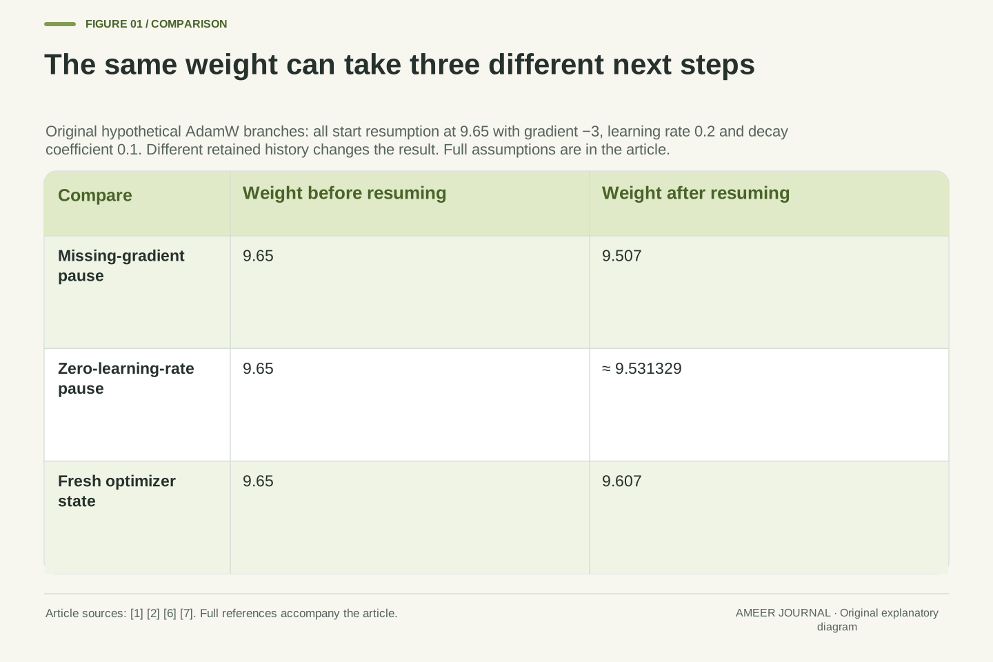
- Three equal weights in the original example become 9.507, about 9.531329 and 9.607 after the same next gradient because their histories differ.
- A continuation record needs matching parameter values, optimizer state, settings and parameter identity.
A pause needs a more precise description
Suppose a model weight has stopped changing during part of a training run. Has its learning process really paused? The answer depends on what happened to the optimizer, the procedure that uses gradients and its own stored information to choose updates. Keeping a weight still for one step does not necessarily keep that stored information still.
A gradient describes how the current loss changes with a small change in a weight. A zero gradient is a numerical result. An absent gradient means there is no gradient object for that parameter at this step. PyTorch documents different optimizer behavior for these cases: a present zero can still take part in an update, while an absent gradient skips the parameter's step [2].
We will compare those cases with setting the learning rate to zero and with starting fresh optimizer history. The examples use invented scalar values and the documented ordinary AdamW equations [1]. They are calculations, not a model-training experiment. Their purpose is to explain why two copies of the same visible weight can take different next steps.
The observable parameter value is only one component of a stateful optimization process. This article separates four interventions: supplying a zero-valued gradient, supplying no gradient, using a zero learning rate for an eligible update, and discarding optimizer state while retaining the parameter. These interventions need not preserve the same state transition.
The reference is PyTorch 2.15 documentation and the v2.15.0 implementation [1][2][6][7]. Scope is ordinary minimizing AdamW with real nonsparse parameters, scalar hyperparameters, amsgrad=False, foreach=False, fused=False, capturable=False and differentiable=False. We exclude AMP, compilation, nonfinite values, hooks and other parameter writers. The selected implementation admits parameters whose gradient is not None.
Our scalar reference uses exact fractions where possible and high-precision decimal square roots where necessary. It does not execute PyTorch or the retrieved implementation. Supplied gradients are hypothetical inputs, not measurements from a dataset. The resulting distinctions concern the declared optimizer transition, without establishing training quality, convergence, speed or bitwise agreement with a tensor backend.
The optimizer remembers more than the last weight
AdamW keeps two running summaries for each participating parameter. One follows the signed gradients, so recent positive and negative values can partly cancel. The other follows squared gradients, so their sign disappears. The algorithm also uses an update count when correcting these summaries for their zero starting values [1]. These are separate pieces of information from the weight itself.
This history explains why a new zero gradient need not produce a zero adjustment. A running summary can remain positive after a new contribution of zero. AdamW also applies weight decay through a separate part of its update [1]. In our positive-weight example, the chosen decay factor reduces the weight even if the new gradient supplies no adjustment.
Think of a saved optimizer record as containing the information needed to interpret the next gradient. PyTorch's optimizer state dictionary stores state per parameter and stores parameter-group settings, including learning rate and weight decay; it does not itself store the parameter values [4]. Both the values and the matching history matter when describing a continuation.
Write the scalar parameter as θ, first moment as m, second moment as v and parameter update count as t. For an eligible gradient g, our non-AMSGrad recurrence is m′=β₁m+(1−β₁)g and v′=β₂v+(1−β₂)g². Increment t and compute m̂=m′/(1−β₁ᵗ) and v̂=v′/(1−β₂ᵗ), using the incremented count [1].
The documented AdamW parameter update is θ′=(1−ηλ)θ−ηm̂/(√v̂+ε), where η is learning rate and λ is the PyTorch weight-decay coefficient [1]. Decay is outside the moment recurrences. A zero g can leave m′ nonzero, and a nonzero ηλ can change θ independently of the adaptive subtraction.
The inspected implementation initializes and retains these states per parameter, adding its state counter to the update list only when its gradient exists [7]. Optimizer.state_dict separately describes per-parameter state and group metadata without saving the parameter values [4]. Thus a weight-only comparison omits variables that the next update actually consumes. This is an accounting distinction, not a suggestion that every stored field changes on every call.
Build one checkpoint with transparent numbers
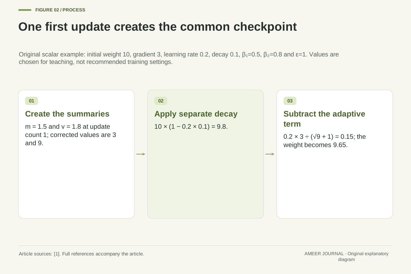
Start with one weight equal to 10 and no previous optimizer history. Choose learning rate 0.2, weight-decay coefficient 0.1, first-summary factor 0.5, second-summary factor 0.8 and the denominator's extra constant equal to 1. These are deliberately simple teaching values. In particular, the extra constant is much larger than the documented default; this is not a suggested training configuration [1].
Supply a first gradient of 3. The running summaries become 1.5 and 1.8. After the algorithm corrects their zero-start effect, the values used in the adjustment are 3 and 9. The square root of 9 is 3, and the extra constant makes the denominator 4. The gradient-based subtraction is therefore 0.2 times 3 divided by 4, or 0.15.
Separately, the decay multiplier is one minus 0.2 times 0.1: 0.98. It changes 10 to 9.8 before the subtraction of 0.15. Our checkpoint is weight 9.65, signed summary 1.5, squared summary 1.8 and update count one. Every comparison below starts from this same checkpoint unless a fresh history is explicitly specified.
Set θ₀=10, m₀=v₀=0 and t₀=0. Choose η=1/5, λ=1/10, β₁=1/2, β₂=4/5 and ε=1. These hypothetical hyperparameters make the arithmetic inspectable and are neither defaults nor recommendations. In particular, ε differs from the cited API's default 10⁻⁸ [1]. All comparisons retain these values except the explicitly changed setting.
For g₁=3, the recurrences give m₁=3/2 and v₁=9/5. Bias corrections yield m̂₁=3 and v̂₁=9. The decay factor is 1−ηλ=49/50. Consequently θ₁=(49/50)10−(1/5)3/(3+1)=49/5−3/20=193/20=9.65.
Retain the complete checkpoint (θ,m,v,t)=(193/20,3/2,9/5,1). We branch from this state rather than sequentially applying every proposed pause to the same object. That branching matters: otherwise one comparison could inherit another's changed history. The gradient values are supplied to the scalar equations, with no claim that a particular loss function or model produced them.
A present zero gradient still changes this weight
First, give the checkpoint a gradient value of zero and keep the ordinary learning rate. The signed summary halves from 1.5 to 0.75. The squared summary becomes 0.8 times 1.8, or 1.44. Both have changed, but neither has become zero. This is the second update, so the corrections must use count two rather than count one.
The corrected summaries are now 1 and 4. Taking the square root of 4 and adding the extra constant gives 3, so the gradient-based subtraction is 0.2 divided by 3: one fifteenth. Decay separately changes 9.65 to 9.457. Subtracting one fifteenth leaves approximately 9.390333, below the original checkpoint weight.
The new gradient was zero throughout that calculation. The change came from retained history and decay, which are part of the documented update [1]. A zero gradient therefore does not establish that this optimizer leaves the parameter unchanged. It also does not establish that training has found a globally best model; it only describes the supplied derivative value for this step.
From the retained checkpoint, set g₂=0 while keeping η=1/5. The new state is t₂=2, m₂=(1/2)(3/2)=3/4 and v₂=(4/5)(9/5)=36/25. The correction denominators are 1−(1/2)²=3/4 and 1−(4/5)²=9/25, giving m̂₂=1 and v̂₂=4.
Apply the two parameter terms separately: the decayed weight is (49/50)(193/20)=9457/1000, and the adaptive subtraction is (1/5)/(2+1)=1/15. Hence θ₂=9457/1000−1/15=28171/3000≈9.390333. Every nonzero contribution is visible even though the newly supplied g₂ is exactly zero.
The formula distinguishes the instantaneous gradient from the optimizer's complete update direction [1]. Historical m contributes after its exponential attenuation; decay contributes outside the moments. This finite example does not imply that every zero-gradient update changes every parameter: zero state, zero weight, zero coefficients or exact cancellation can alter the outcome. It disproves the unconditional inference from g=0 to θ′=θ.
Remove one cause at a time
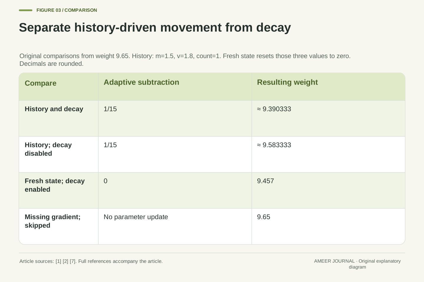
To see the two causes clearly, repeat the zero-gradient calculation from the original checkpoint while switching off weight decay. Keep the history. The one-fifteenth subtraction remains, so the weight becomes about 9.583333. The weight still moves because the optimizer still remembers the earlier positive gradient.
Now try a separate branch with the same weight, 9.65, but fresh zero summaries and count zero. Keep weight decay and supply a zero gradient. The summaries remain zero, so the gradient-based subtraction is zero. Decay alone changes the weight to 9.457. This branch deliberately removes history; it is not what an ordinary missing-gradient step does.
These branches identify two independent explanations for movement in our original example. With fresh zero summaries and repeated zero gradients, the chosen decay factor would multiply the weight by 0.98 on each participating update. The number of such updates therefore matters. Skipping a parameter's update does not apply the same repeated multiplication, even if the surrounding training loop continues running.
The first intervention changes only λ to zero at the common checkpoint. For g=0, m′=3/4, v′=36/25 and t′=2 remain unchanged from the previous calculation. The adaptive subtraction is still 1/15, so θ′=193/20−1/15=115/12≈9.583333. Momentum-derived movement survives removal of decay.
The second intervention retains θ=193/20 but replaces state with m=v=0,t=0. With g=0 and the original nonzero λ, the moments remain zero, their corrections are defined, and ε=1 keeps the denominator positive. The new weight is solely (49/50)(193/20)=9457/1000=9.457. This is a counterfactual state reset, not an implicit effect of zero_grad [1][2].
For fresh zero moments, constant η and λ, and n eligible zero-gradient updates, the recurrence reduces to θₙ=θ₀(1−ηλ)ⁿ. Our retained arithmetic checks this identity through twelve updates. This statement requires the specified initial state and repeated zero gradients; it cannot be substituted for the history-bearing case, where the adaptive term generally persists.
An absent gradient skips the parameter without erasing its past
Return to the original checkpoint. This time the parameter's gradient is absent, represented by None in PyTorch. The cited zero_grad documentation distinguishes that state from a tensor filled with zeroes [2]. In the inspected AdamW implementation, only parameters with an existing gradient are added to the update's parameter and state lists [6][7].
Under that ordinary update path, our parameter stays at 9.65. Its summaries stay at 1.5 and 1.8, and its update count stays at one. No decay is applied to this skipped parameter. Other eligible parameters can still be processed during the same optimizer call; the statement concerns the parameter we are following.
The old history has been preserved, not forgotten. If a later step supplies another gradient, the optimizer can continue from that history. This is why a skipped update and a fresh optimizer are different choices even when both leave the current weight at 9.65. The next gradient provides a way to make their difference visible.
For the v2.15.0 implementation, AdamW inherits Adam while enabling decoupled_weight_decay [6]. Adam's group initialization adds a parameter and its m,v,step state only under the condition p.grad is not None; the subsequent update consumes those eligible lists [7]. None is therefore a participation condition, not a numeric value fed into the moment recurrences.
From our checkpoint, an absent gradient leaves (θ,m,v,t)=(193/20,3/2,9/5,1). The selected update applies neither decay nor moment attenuation nor counter increment to this parameter. Repeating that absence does not age its moments through zero-gradient steps. This is consistent with the documented distinction between a zero-gradient step and a skipped step [2].
The conclusion assumes no separate mutation of the parameter or state. It also does not say that the entire optimizer call is skipped: other parameters can have gradients. Most importantly, skipping does not clear existing state. On re-entry, the retained moments and count still influence the bias corrections and parameter update, unlike reinitializing an optimizer's state at the same θ.
A zero learning rate can preserve the weight while changing the history
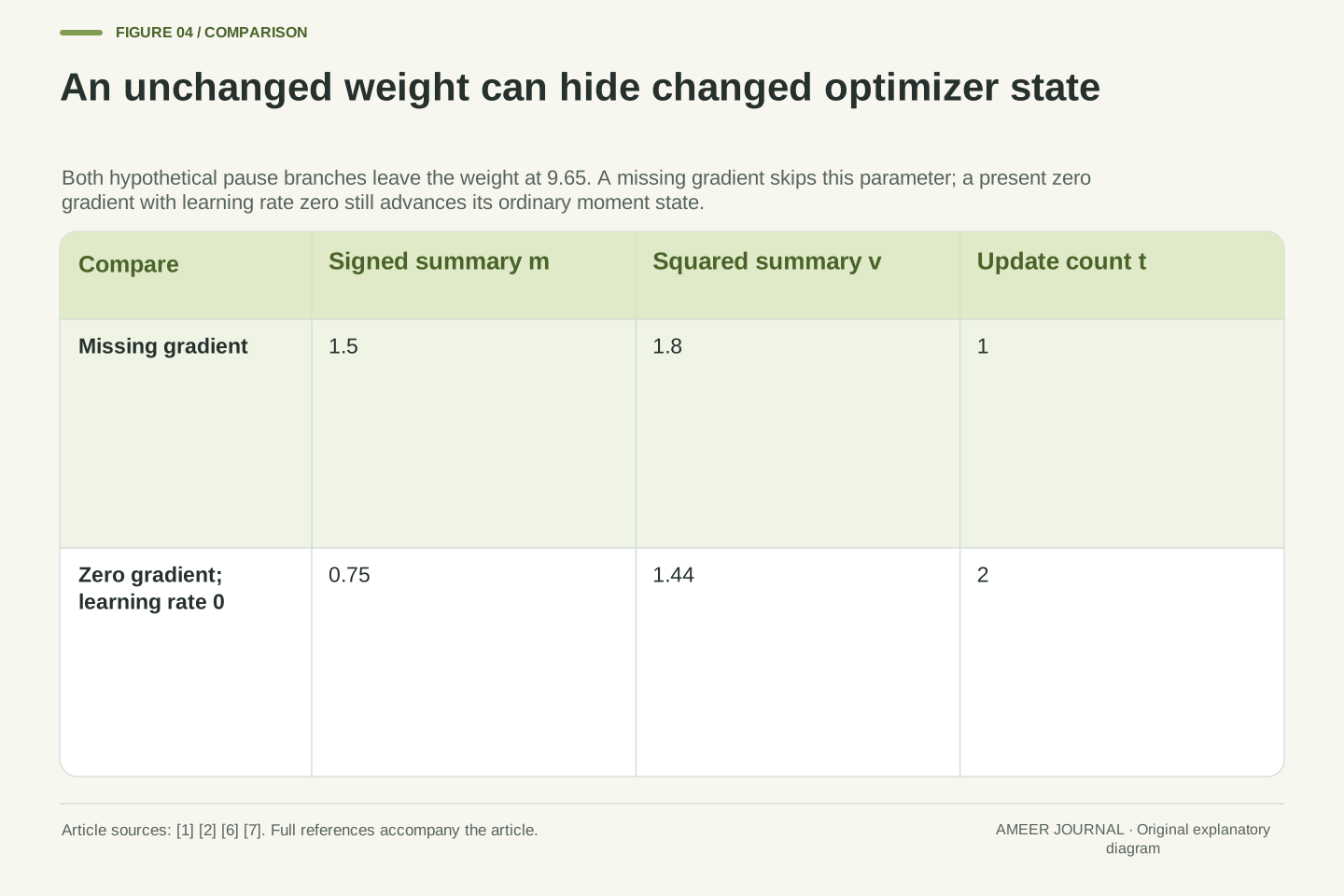
There is another way to keep the weight still in our example. Give the parameter a present gradient of zero, but use learning rate zero for that update. Both the decay change and the gradient-based change to the weight are multiplied by the learning rate, so the weight remains 9.65.
The stored summaries do not use the learning rate in their own recurrences [1]. They still become 0.75 and 1.44, and the count advances to two in the ordinary implementation path [7]. The visible weight now matches the skipped-gradient branch, but the optimizer history does not. Looking only at saved weights would miss that difference.
Restore the ordinary learning rate later and that changed history can affect the next adjustment. Setting the learning rate to zero is therefore a precise intervention with a particular effect, rather than a complete description of pausing all learning-related state. This example does not extend that claim to every optimizer implementation, every numerical mode or an update containing nonfinite values.
Apply an eligible g=0 update to the common checkpoint with η=0 while preserving β₁,β₂,λ and ε. The moment state becomes m′=3/4,v′=36/25,t′=2, exactly as in the normal-learning-rate zero-gradient branch. However, θ′=(1−0·λ)θ−0·m̂/(√v̂+ε)=θ=193/20.
This distinction is visible in both the documented equations and the selected ordinary source path: the counter and moment operations occur independently of the scalar learning-rate factor used for the parameter update [1][7]. We deliberately exclude capturable, differentiable, fused and nonfinite paths rather than infer their behavior from this scalar reasoning.
The resulting state is (193/20,3/4,36/25,2), whereas the missing-gradient branch retains (193/20,3/2,9/5,1). Equal θ does not imply equal m,v,t. Our calculation also checks weight preservation and the stated moment/counter recurrences for 96 finite combinations of specified coefficients, starting values and gradients. Those are mathematical reference checks, not execution tests of the retrieved library.
The same next gradient exposes three different histories
Take three branches that all now have weight 9.65. One skipped the pause update and kept its earlier history. Another took the zero-gradient update with learning rate zero. The third starts fresh history at the same weight. Restore the ordinary learning rate of 0.2 and give every branch the same next gradient: minus 3.
The skipped branch reaches 9.507. The zero-learning-rate branch reaches about 9.531329. The fresh-history branch reaches 9.607. Their starting weight, current gradient and current settings are equal; their past optimizer states differ. The negative gradient creates an upward adaptive adjustment here, but the size depends on that retained history as well as the current input.
This comparison is why checking that a supposedly paused weight stayed still can be necessary without answering the whole question. It establishes what happened to the parameter during the pause, but it does not establish how the parameter will resume. A clear experiment records whether history was preserved, advanced or deliberately reset, rather than treating all three outcomes as the same kind of freeze.
Resume the three equal-weight states with g=−3, η=1/5 and λ=1/10. The skipped branch advances to t=2,m=−3/4,v=81/25, giving corrected moments −1 and 9. Thus θ′=9457/1000−(1/5)(−1)/(3+1)=9507/1000=9.507.
The zero-learning-rate history instead advances to t=3,m=−9/8,v=369/125. Its corrected moments are −9/7 and 369/61. Therefore θ′=9457/1000+(9/35)/(√(369/61)+1)≈9.531329311. The fresh-history branch has its first update, corrected moments −3 and 9, and θ′=9457/1000+3/20=9607/1000=9.607.
These are three transitions with equal starting θ, equal present g and equal current hyperparameters. The distinction is entirely in m,v,t. Decimals are rounded from the retained exact expressions or high-precision evaluation; no measured training trajectory is implied. The construction demonstrates that a weight-preserving pause can change subsequent optimization without requiring a change in the visible checkpoint weight itself.
The zero-gradient issue also appears in ordinary momentum
AdamW's details are useful, but stored history is not unique to it. PyTorch's ordinary stochastic gradient descent optimizer can use a momentum buffer that carries part of a previous update forward [3]. A simpler example makes the same zero-versus-absent distinction without AdamW's two summaries or bias corrections.
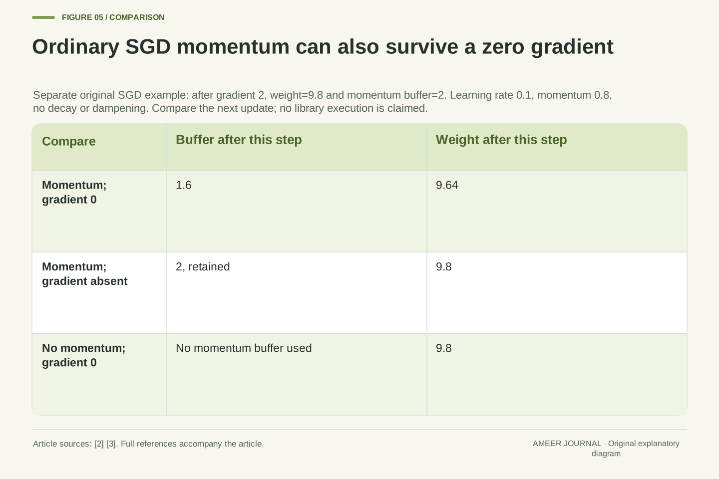
Start a separate weight at 10, choose learning rate 0.1 and momentum factor 0.8, and use no weight decay or dampening. A first gradient of 2 creates a buffer of 2 and moves the weight to 9.8. With a present zero gradient next, the buffer becomes 0.8 times 2, or 1.6. Subtracting 0.1 times 1.6 moves the weight again, to 9.64.
If that second gradient is absent, the ordinary parameter update is skipped and the weight stays 9.8 [2]. With momentum switched off in a separate comparison, a present zero gradient also leaves the weight at 9.8. Those equal weights arise for different reasons. Name the optimizer and its state rule before interpreting a zero-gradient observation.
For a separate SGD fixture, take learning rate a=1/10, momentum μ=4/5, zero dampening, zero weight decay and nesterov=False. PyTorch documents initializing the first momentum buffer to the first gradient, rather than applying dampening to a pre-existing zero buffer [3]. With θ₀=10,g₁=2, this yields b₁=2 and θ₁=10−(1/10)2=49/5=9.8.
For a second present gradient g₂=0, b₂=μb₁+g₂=8/5 and θ₂=49/5−(1/10)(8/5)=241/25=9.64. An absent gradient instead skips the parameter step [2]. In the separate no-momentum, no-decay case, a present zero gradient gives zero subtraction and also leaves θ=9.8.
The equal parameter values in the last two cases do not establish equal internal configurations. The cited SGD notes also distinguish its momentum convention from implementations that place learning rate inside the velocity recurrence [3]. Our calculation follows the named convention and does not transplant its buffer values or pause behavior to another optimizer solely because it also uses the word momentum.
Keep the decay rule and its coefficient convention together
Weight decay and a penalty added to the loss are related ideas, but their implementation matters. The original AdamW paper explains why adding a squared-weight penalty into an adaptive gradient calculation is generally different from applying decay separately [5]. A penalty added to the gradient can also enter the optimizer's historical summaries.
Our calculations use the PyTorch AdamW rule, where the decay multiplier is one minus learning rate times weight-decay coefficient [1]. With our chosen settings, that is 0.98. This is why reducing the learning rate to zero removes the decay change for the particular update we studied.
Be careful when comparing equations across sources. The paper's opening weight-decay equation uses a coefficient that directly represents the fraction removed per step [5]. Its symbol is not automatically the same numerical setting as the PyTorch argument. Here the direct fraction is 0.02, while the PyTorch weight-decay coefficient is 0.1. Keeping the complete formula prevents a matching name from hiding different quantities.
The original decoupled-weight-decay paper distinguishes a separate parameter shrinkage from adding an L2 penalty gradient before adaptive processing [5]. In its Appendix A argument, a non-scalar preconditioner generally prevents a single ordinary L2 coefficient from reproducing a uniform decay operator for all parameter vectors. We use that mechanism distinction without adopting its historical benchmark claims.
The present fixture specifically uses PyTorch θ′=(1−ηλ)θ−ηm̂/(√v̂+ε), with λ excluded from m and v [1]. By contrast, the paper's opening Equation 1 writes θnext=(1−λpaper)θ−α∇f. For this one-step decay comparison, λpaper=ηλPyTorch; the matching symbols alone do not justify equating the numeric coefficients.
Our values give λpaper=0.2×0.1=0.02 and shrinkage factor 0.98. This convention explains the zero-learning-rate result without claiming that every method called decoupled decay uses identical schedule placement. The paper also presents color-coded alternative algorithms; combining their penalty and decay terms would describe a different update. Preserve the implemented formula, coefficient meaning and schedule when comparing pause behavior.
Check the parameter that actually reaches the optimizer
The example follows one complete scalar parameter. In a real model, a parameter may contain many values. A gradient tensor can exist while some of its entries are zero. That is different from having no gradient object for the entire parameter. The inspected optimizer checks whether the parameter's gradient exists before admitting it to the update [7].
This also makes the timing of a change important. Saying that a parameter should receive no new gradient does not describe an older gradient object that may already be present. PyTorch's zero_grad documentation explains the effect of setting gradients to None before a backward pass [2]. A clear record distinguishes the gradient object actually supplied from the intention to stop computing new derivatives.
Choose an observable question. Are the parameter values unchanged? Are the optimizer's summaries and count unchanged? Does resuming produce the same update? These require different comparisons. The present article addresses optimizer state; model training modes and other mutable buffers are separate controls. An observation about one of these objects cannot establish that every part of the model has paused.
Eligibility in the inspected path is tested at the parameter-tensor level through p.grad is not None [7]. A zero coordinate inside an existing gradient tensor does not remove the containing parameter from that list. Our scalar fixture therefore represents one whole parameter, not a claim that None can independently skip arbitrary coordinates while preserving the rest of a tensor's update.
The source inclusion test also clarifies a stale-gradient boundary: an existing gradient can remain eligible even if the operator's intention is to prevent future gradient computation. Gradient-reset semantics, future differentiation choices and optimizer membership are distinct records [2][7]. This is a reason to inspect actual participation, not a blanket instruction to clear gradients during an accumulation scheme.
For the selected optimizer, compare captured θ and m,v,t before and after the intended pause, together with the supplied gradient status and hyperparameters. A parameter equality check tests one property; state equality tests another. A continuation check tests the resulting transition. These distinctions do not cover training-mode modules, persistent model buffers or unrelated writers, which require their own declared scope.
A reproducible continuation pairs values with the matching state
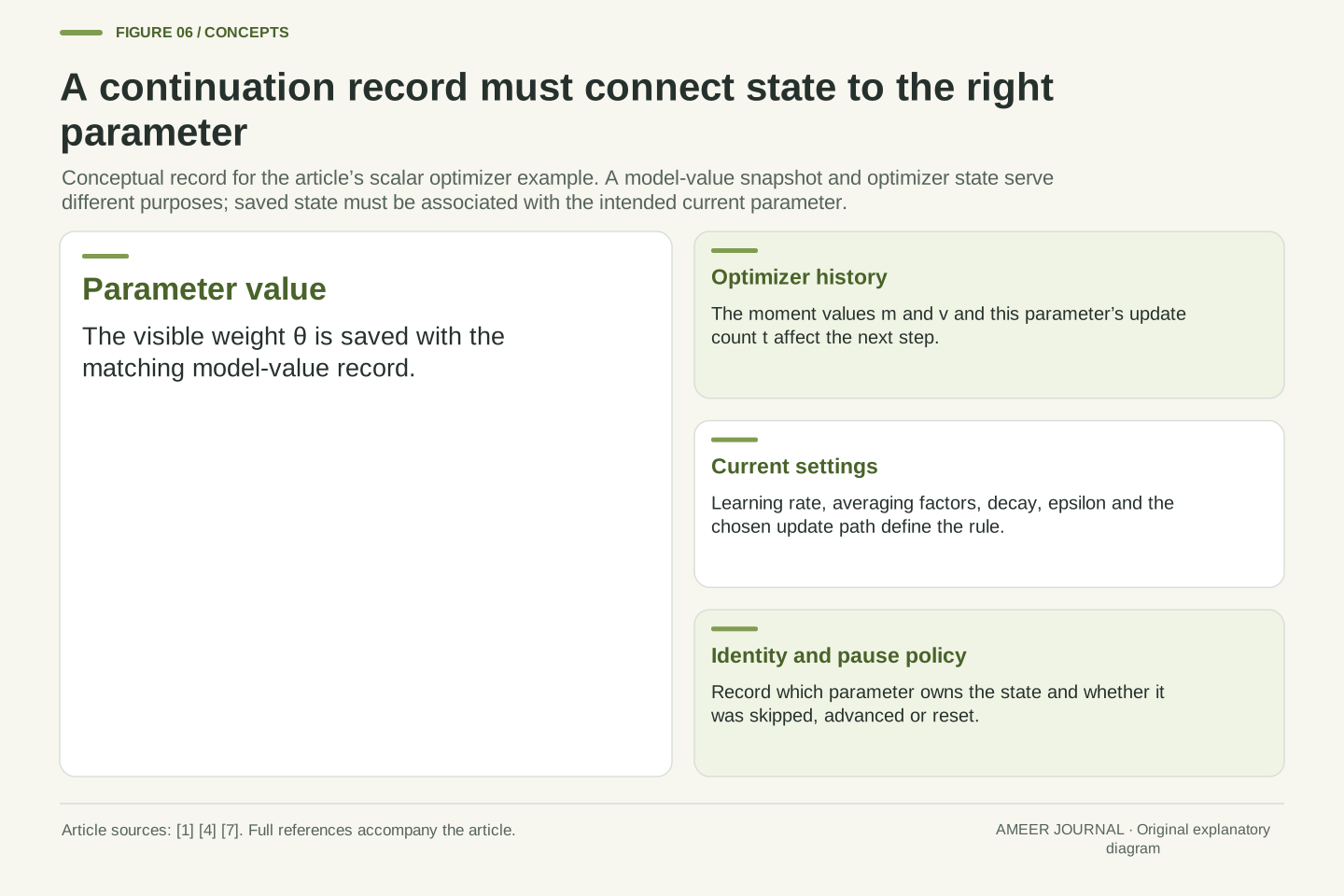
A useful continuation record pairs the parameter values with their matching optimizer state and settings. For our example that means the weight, both summaries, the update count, the learning rate, the two averaging factors, decay and the denominator's extra constant. It also records which pause was applied, so the next result can be explained.
Restoring state requires the right association with the current parameters. PyTorch documents that saved optimizer identifiers are matched to current parameter groups in order, without an additional verification of that match [4]. Its loading notes also explain that saved parameter names do not by themselves control the loading process [1]. A file containing history is not enough if that history is attached to the wrong parameter.
The worked result remains specific and useful: zero gradients can preserve momentum-derived movement, missing gradients can preserve old history without advancing it, and zero learning rate can keep weights still while history advances. Equal saved weights therefore do not guarantee equal next updates. Recording the complete transition makes a pause understandable without pretending that its arithmetic proves model quality or a successful training outcome.
For this fixture, a continuation record includes θ,m,v,t,β₁,β₂,η,λ,ε, parameter identity and the pause intervention. Distinguish a state reset from an update skip and from an eligible zero-learning-rate update. Optimizer.state_dict contains state and parameter-group metadata but not parameter values, so it cannot replace a matching model-value record [4].
The cited loader semantics map saved parameter IDs to current parameter groups by ordering, without additional verification, and the AdamW loading notes say that saved parameter names alone do not determine the loading process [4][1]. Correct state association is part of resumption. These observations are not a complete guarantee of experiment reproducibility, which can involve other execution state outside this scalar model.
Our independent branches establish the concrete boundary: θ=9.65 with three different histories becomes 9.507, approximately 9.531329 or 9.607 after the same next gradient under the same current settings. A weight-only snapshot cannot distinguish those histories. Preserve the state variables actually consumed by the next transition, and keep conclusions about optimizer behavior separate from claims about model accuracy or training performance.
Sources & further reading
Explore the references behind this guide. External pages may change after our review.
- AdamW — PyTorch 2.15 documentationPyTorch · Accessed 7 Nov 2026
- torch.optim.Optimizer.zero_grad — PyTorch 2.15 documentationPyTorch · Accessed 7 Nov 2026
- SGD — PyTorch 2.15 documentationPyTorch · Accessed 7 Nov 2026
- torch.optim.Optimizer.state_dict — PyTorch 2.15 documentationPyTorch · Accessed 7 Nov 2026
- Decoupled Weight Decay RegularizationLoshchilov and Hutter / University of Freiburg / arXiv · Accessed 7 Nov 2026
- pytorch/torch/optim/adamw.py at v2.15.0 · pytorch/pytorch · GitHubPyTorch · Accessed 7 Nov 2026
- pytorch/torch/optim/adam.py at v2.15.0 · pytorch/pytorch · GitHubPyTorch · Accessed 7 Nov 2026
Article updated 7 Nov 2026.
Found something we should revisit?
Good explanations get better with thoughtful feedback.