What you’ll take away
- A mean credited speed reduction does not uniquely identify how many contacts were avoided.
- A reporting convention can assign zero impact speed to avoidance without proving a complete stop.
- An average across all coded records differs from a mean among contact cases only.
- Rounding, trial mixtures and missing results must retain their own definitions and denominators.
- The original finite examples explain reports; they do not estimate real-world crash probabilities.
An average and an avoided-contact count answer different questions
A report says an automatic emergency braking system achieved an average speed reduction of 25 kilometres per hour. Does that mean it avoided half the possible collisions, slowed equally in every trial, or left every contact at the same speed? None of those conclusions follows from the average alone. Automatic braking can aim to avoid a collision or reduce its severity, while a warning is a different function. NHTSA keeps those purposes distinct. [3] The result therefore needs an outcome record as well as a number.
We will compare invented records with the same average and different contact outcomes. Every example is a paper calculation, with no vehicle, controller or driving experiment behind it. The records will make their reference speed, outcome labels and reporting rules explicit. They are not an official rating calculation. Their value is practical: when you read a test summary, you can ask which events it counted, which values it averaged and which information disappeared in the summary.
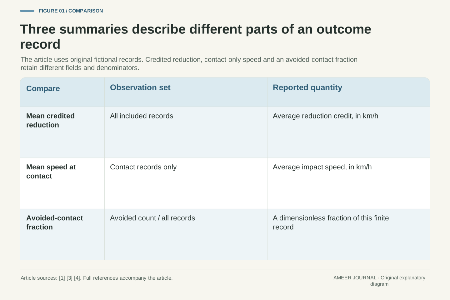
A mean reduction is a statistic over numerical records; an avoidance count is a statistic over outcome labels. They need not be recoverable from each other. NHTSA distinguishes forward-collision warning from intervention and describes automatic braking in terms of avoidance or mitigation. [3] Consequently, an intervention result has several potentially relevant observables: whether contact occurred, the speed associated with contact, the credited reduction and the particular conditions represented. One scalar does not automatically encode them all.
The following constructions use finite stipulated records rather than empirical samples or a simulated braking controller. We hold a reference speed fixed within each comparison, define an outcome-coding rule and independently retain the contact indicator. This lets us examine what an arithmetic mean identifies without supplying an unmeasured response delay, deceleration trajectory or injury model. The central question is information loss in a result summary, not whether a specific vehicle would perform either constructed pattern.
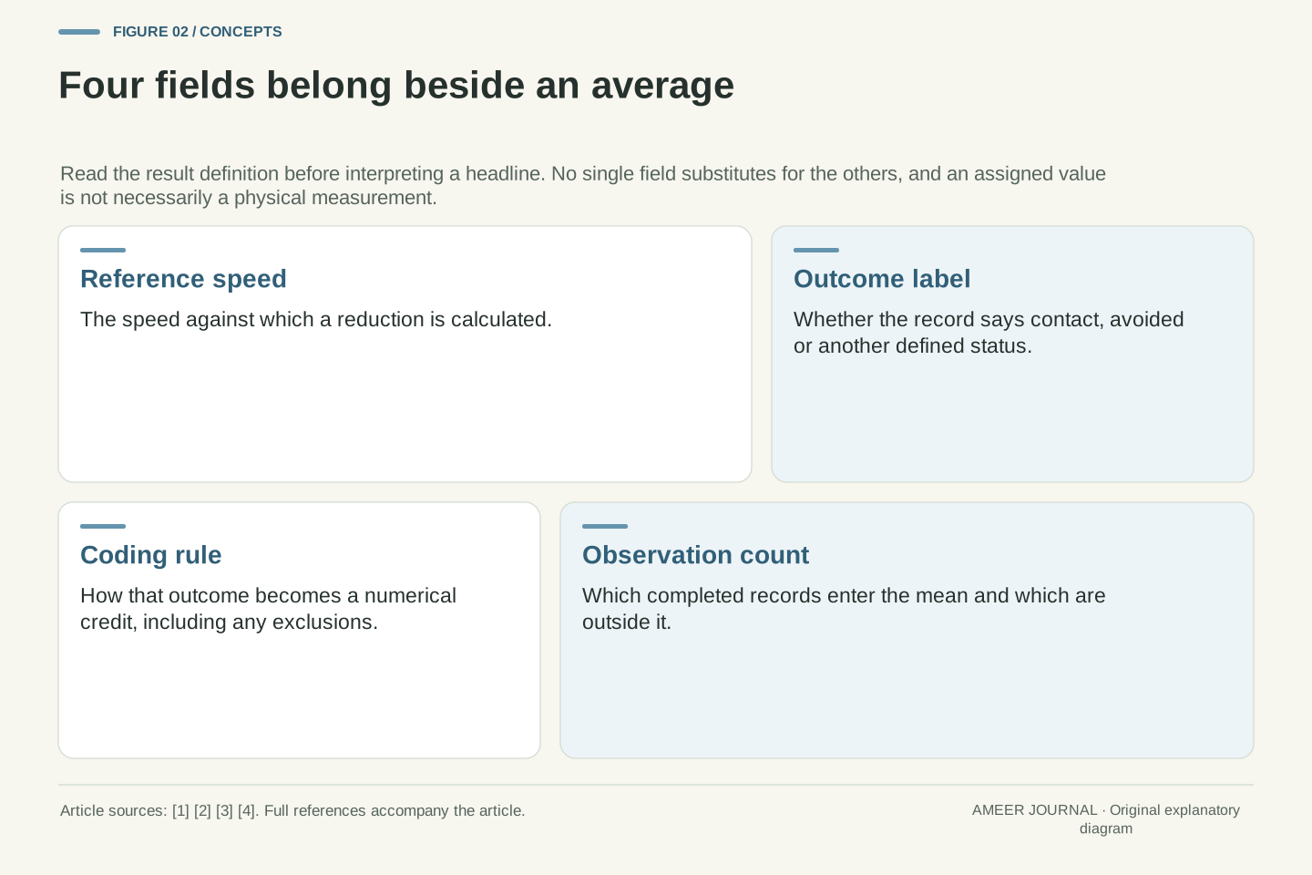
First check whether the number is a measurement or an outcome credit
The April 2025 Version II IIHS front-crash-prevention protocol uses a particular reporting rule. Avoiding contact while remaining in an unoccupied travel lane receives zero assessed impact speed, regardless of the countermeasure used. A contact trial instead compares impact speed with its pre-intervention reference. Automatically moving, or attempting to move, into an occupied lane or off the marked road receives no reduction credit. [1] Those qualifications belong to the result; the words speed reduction do not replace them.
An assigned zero impact speed in a no-contact case is therefore not proof that the vehicle came to a complete stop. There was no impact at which to measure that value. This matters before interpreting an average as an ordinary record of how much every vehicle slowed. Our examples below use a simpler, explicitly stated braking-only account. They retain a separate avoided or contact label, so a reporting convention cannot silently become a claim about the vehicle's actual motion.
The retrieved IIHS protocol is Version II, April 2025. Its qualifying no-contact outcome, within an unoccupied travel lane, is assigned zero impact speed regardless of countermeasure. Contact cases use impact speed relative to the specified pre-intervention speed; occupied-lane or off-road automatic movement or attempted movement receives zero reduction credit. [1] This is a defined assessment mapping, not an unrestricted identity between a credited reduction and a literal change of speed along every trajectory.
An encoded zero for an avoided contact must therefore be distinguished from an observed zero velocity. The no-contact case has no physical impact-speed observation. We use that distinction to motivate a separate teaching model, not to reproduce the full protocol. Its later assumptions exclude automatic steering and those lane exceptions, keep the reference speed exact and record the outcome label independently. A reader should preserve the corresponding definitions in a real report before comparing, converting or averaging its fields.
Build one record before calculating a summary
Imagine six completed, equally weighted records under the same stated condition. Each has an exact reference speed of 50 kilometres per hour. In this teaching account, a record either says avoided, meaning no contact occurred, or says contact and supplies a positive impact speed. For an avoided record, assign an outcome speed of zero for arithmetic. For a contact record, use its stated impact speed. Subtract that outcome speed from 50 to obtain the credited reduction. All credits are between zero and 50.
For example, a contact at 30 kilometres per hour receives a reduction of 20. An avoided contact receives the full credit of 50. Keep the words beside the numbers: the zero assigned to an avoided contact is not a measured impact. To find the mean reduction, add the six credits and divide by six, following the ordinary arithmetic-mean definition. [4] This procedure gives one summary of the complete record; it does not replace the labels or make six trials an official test sequence. The reference also matters: a reduction of 25 from 50 leaves a coded outcome speed of 25, whereas the same reduction from 70 leaves 45. All those speeds are in kilometres per hour.
For each of n=6 fictional records, specify the same reference V=50 km/h and an outcome indicator a_i, equal to one for avoidance and zero for contact. Set the coded outcome speed v_i*=0 when a_i=1. For a contact record, v_i* is the assigned positive impact speed, bounded by V. Define credited reduction d_i=V−v_i*, so 0≤d_i≤V. No acceleration above the reference, exceptional lane result or missing observation enters this initial fixture. The labels refer to the outcome of each separate record.
The numerical mean is m=(Σd_i)/n, consistent with the arithmetic definition. [4] A contact at 30 km/h gives d_i=20 km/h; an avoided contact gives d_i=50 km/h by convention. The star on v_i* marks the coded field: averaging it across all records does not produce a contact-only impact-speed mean. The outcome indicator remains available for that separate calculation. The fixed reference and equal record weights are substantive assumptions. For example, a 25 km/h credit from a reference of 50 leaves a coded outcome speed of 25 km/h; the same credit from 70 leaves 45 km/h. The credit alone does not identify the residual without its reference.
Two complete logs can share the same average
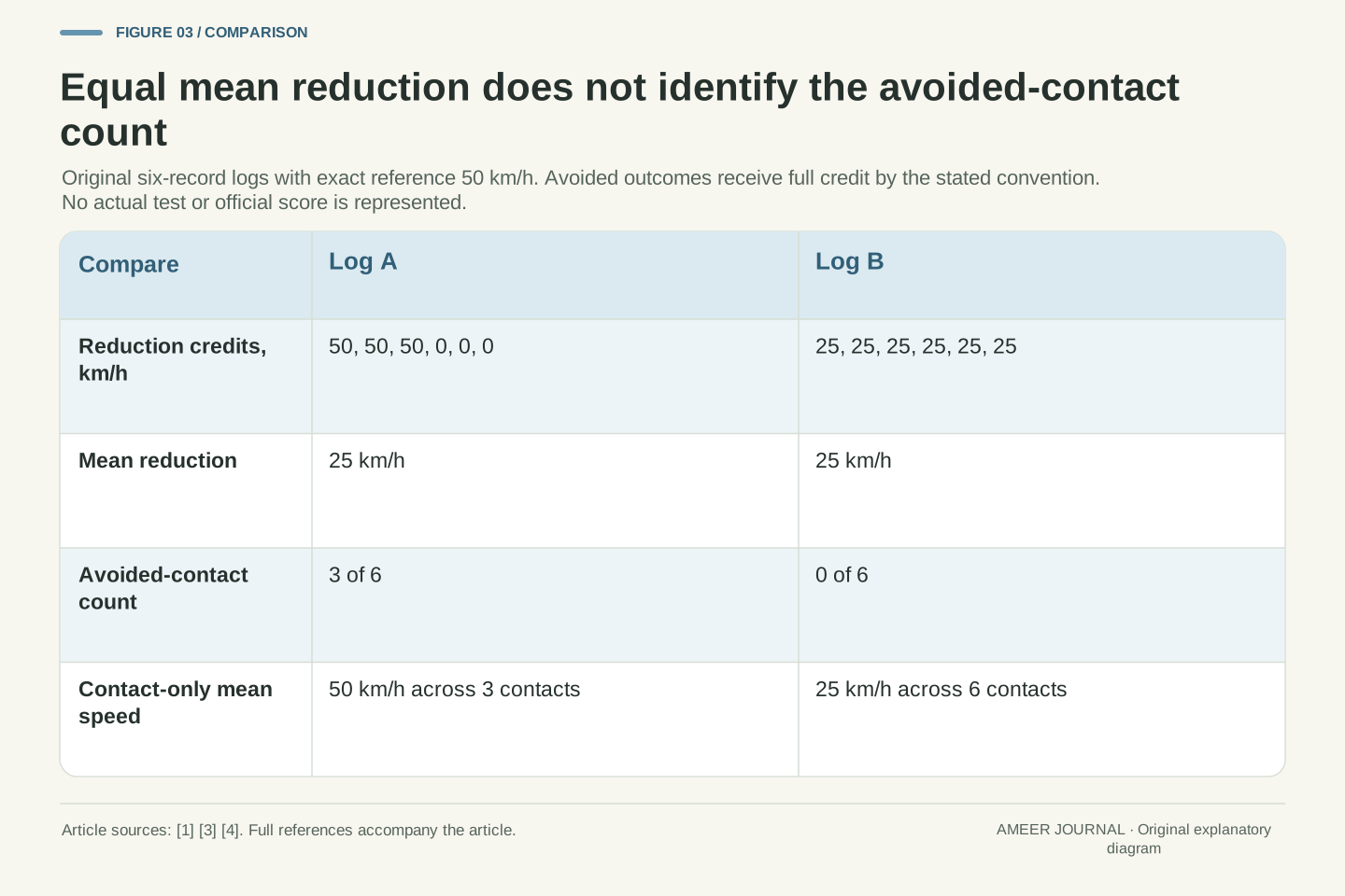
Log A contains three avoided contacts and three contacts at 50 kilometres per hour. Its reduction credits are 50, 50, 50, 0, 0 and 0. Their sum is 150, and dividing by six gives a mean reduction of 25 kilometres per hour. Log B contains six contacts, each at 25 kilometres per hour. Its credits are 25, 25, 25, 25, 25 and 25. They also sum to 150 and average 25. The headline number is identical even though the outcome pattern is different. Neither list is a time sequence within one braking event.
A avoided three contacts out of six; B avoided none. Conversely, the contacts that remain in A occur at a greater speed than the contacts in B. Those statements can both be true. The logs have different strengths under different questions, so their shared mean is not a complete ranking. Keeping the six rows makes that visible immediately. Replacing them with one average removes the distinction between a mixture of full credits and zero credits and a set of equal partial credits.
Let the reduction vector for A be (50,50,50,0,0,0) km/h, with the first three entries labelled avoided and the last three labelled contact. Let B have reduction vector (25,25,25,25,25,25) km/h, all labelled contact. Both sums are 150 km/h across six records, and both arithmetic means are 25 km/h. Their coded outcome-speed vectors are (0,0,0,50,50,50) and (25,25,25,25,25,25) km/h respectively. Every entry describes a separate completed record; reordering entries changes neither mean nor count.
The avoidance counts are k_A=3 and k_B=0, giving finite-record fractions 1/2 and 0. Neither vector is reconstructed from the shared mean; each is an independently stipulated example consistent with it. The construction proves non-uniqueness: m=25 km/h does not determine k. It also shows why selecting one favourable component does not establish a comprehensive comparison. A contains more avoided contacts but higher speeds among its contact cases. No injury or all-conditions performance ordering has been supplied by these records.
Changing the denominator changes the question
Now ask for the average speed among contacts that actually occur in the invented logs. A has three such rows, all at 50 kilometres per hour, so its contact-only mean is 50. B has six contact rows, all at 25, so its contact-only mean is 25. The denominator has changed from six total records to the number of contact records. A's three avoided rows are not contact measurements of zero; they are outside this particular average. If all rows were avoided, there would be no contact-only mean to report.
If instead you average the coded outcome speeds across all six rows, both logs give 25. That calculation includes A's three assigned zeros. The two calculations are useful for different descriptions, provided their names and denominators remain visible. Saying simply average impact speed would blur them. A table that reports the avoided count alongside the contact-only mean makes clear why one log has fewer contacts and a larger mean among the contacts that remain.
The all-record coded outcome mean obeys mean(v*)=V−m=25 km/h for both A and B because V is common to every record. The contact-only mean is c=(Σ over a_i=0 of v_i*)/(n−k), provided n−k>0. Thus c_A=150/3=50 km/h and c_B=150/6=25 km/h. The numerators happen to match, but the observation sets and denominators differ. A smaller conditional mean can coexist with a larger number of contacts. The calculation has changed its conditioning set, not corrected an arithmetic error.
In this fixture, mean(v*)=(1−k/n)c because avoided records contribute coded zeros. For A, (1−1/2)×50=25; for B, (1−0)×25=25, with speed units retained. The same all-record mean can therefore arise through different avoidance fractions and different conditional means. If every record were avoided, the contact-only mean would be undefined rather than a measured zero. A report should retain that absence of a conditioning set instead of manufacturing a contact measurement.
Another centre number still cannot recover the lost rows
Perhaps the median would recover what the mean missed. The median is the middle value after sorting, using the average of the middle two values when there is an even number of observations. [4] Sort A's reduction credits as 0, 0, 0, 50, 50, 50. Its middle pair is 0 and 50, so the median is 25. B's middle pair is 25 and 25, also giving 25. These two logs share both their mean and their median. The central number alone still leaves the extreme rows hidden.
Their spread is different. A's smallest and largest credits are zero and 50, a range of 50 kilometres per hour. Every B credit is 25, so its range is zero. That extra description separates these particular logs, but it is still a description of numerical values. The contact labels remain the direct answer to how many contacts were avoided. Choosing a different summary does not remove the need to state which aspect of the record you want to understand.
For an even count, the median averages the two central sorted observations. [4] A's sorted reductions have third and fourth values 0 and 50 km/h; B's are both 25 km/h. Both medians are consequently 25 km/h, matching their means. Adding this second location statistic does not separate the two original outcome records. Neither statistic retains the allocation of credits across all six rows. In A, the median of 25 km/h does not even occur as an individual credited reduction; a middle-pair average need not be a listed observation.
The numerical ranges are 50 km/h for A and zero for B. Those values separate this chosen pair, but do not establish a universal recipe for reconstructing a trial history from a few statistics. A statement about an avoided-contact count should use the outcome field and its defined denominator directly. Likewise, a statement about worst observed contact speed should retain the contact subset. A summary becomes useful when its observable is named, rather than when it is treated as a substitute for every discarded field.
The mean can bound the count without identifying it
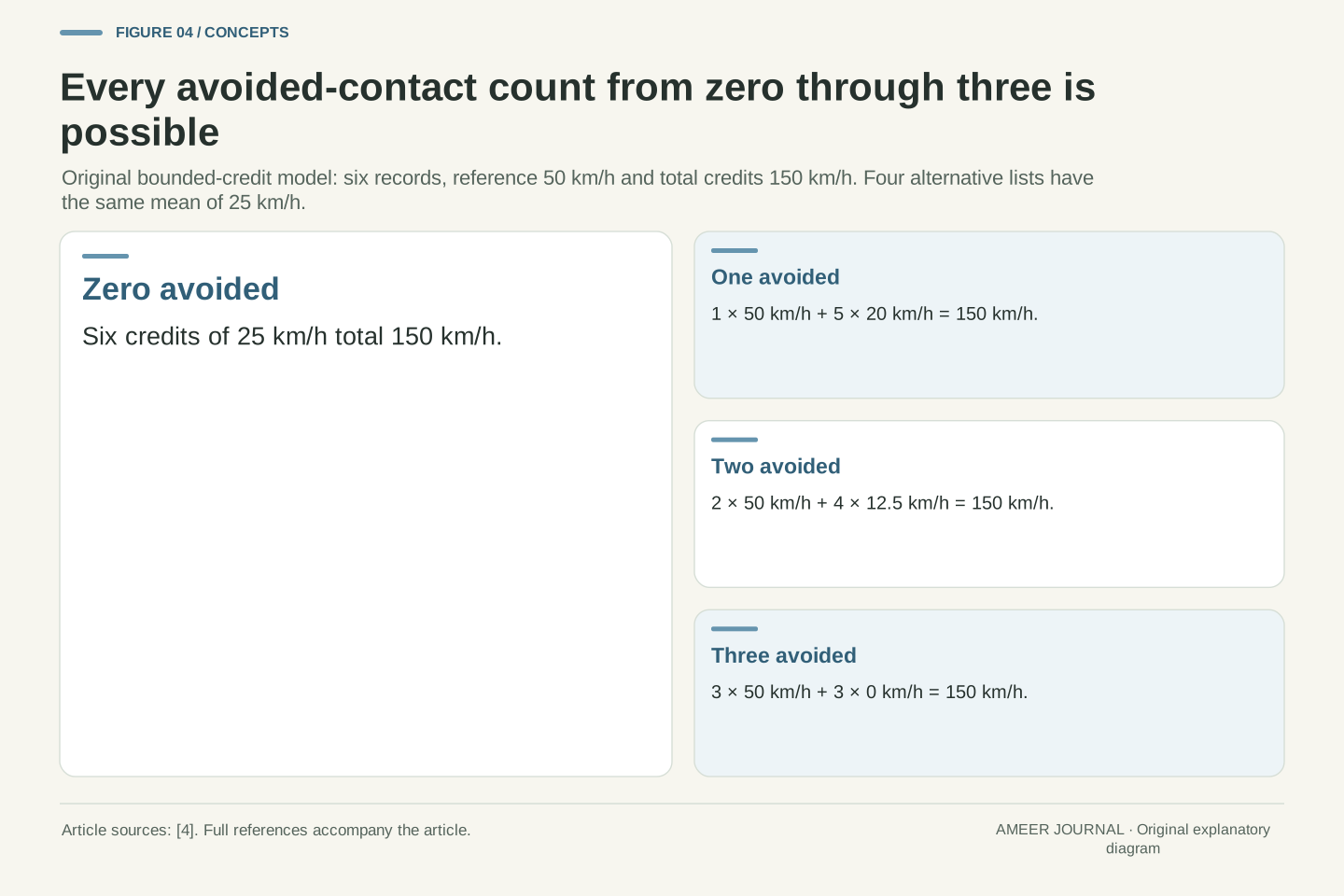
The shared average still tells us something. Six credits averaging 25 add to 150. Each avoided contact contributes a full credit of 50, and every other credit is nonnegative. Four avoided contacts would already contribute 200, too much for that total. There can therefore be at most three avoided contacts in this particular record. The mean rules out some counts even though it does not choose one remaining count. This conclusion uses the nonnegative-credit rule; dropping it would remove the argument.
All four counts from zero through three are possible. Zero avoided contacts can use six credits of 25. One can use one 50 and five 20s. Two can use two 50s and four 12.5s. Three can use three 50s and three zeros. Every list sums to 150 and obeys the same bounds. These are four alternative complete records, not four stages of improvement. The range zero to three is an exact consequence of the supplied information, not a prediction about another test.
With k avoided records, their contribution to Σd_i is kV. Nonnegative credits in the remaining records imply kV≤nm, hence k≤floor(nm/V). For n=6, m=25 km/h and V=50 km/h, the upper bound is three. This is a deterministic feasibility bound over the stipulated finite record. It is not a confidence interval, a sampling-error estimate or a bound on real-world collision probability. Allowing negative credits would change the feasible set, because they could offset additional full credits.
For each k in {0,1,2,3}, assign k full credits and make every remaining credit equal to (150−50k)/(6−k) km/h. The remaining values are 25, 20, 12.5 and 0 km/h respectively. All are below the full credit and within the permitted interval, so the construction has exactly k avoided records and the required total. Attainment at every integer count establishes the complete feasible count set here. A single possible record would prove ambiguity; these four additionally show its exact finite extent.
A displayed maximum need not be an exact maximum
Consider a separate invented display that rounds a mean to the nearest whole kilometre per hour. Give each of six contact records an impact speed of 0.4 kilometres per hour from the same reference of 50. Each reduction is 49.6, so the exact mean is 49.6. The display shows 50, while the record still contains six contacts and zero avoided contacts. This separate rounding rule is ours for the example; it is not the IIHS protocol's reporting calculation.
Compare that with an exact mean of 50 under our bounded-credit rules. Because no individual credit can exceed 50, every credit would then have to equal 50. A lower one could not be balanced by a higher one. Under our explicitly assigned outcomes, that would mean every record was avoided. The word exact is doing real work. A rounded label, the underlying numerical mean and the recorded event labels should remain separate when a report is copied into a comparison table.
Use a separate display rule round(x)=floor(x+1/2) for nonnegative speeds expressed numerically in km/h. Six contact records with v_i*=2/5 km/h have d_i=248/5 km/h=49.6 km/h. Their exact mean is 49.6 km/h and their displayed mean is 50 km/h, but k=0. This stipulated nearest-integer display is not the IIHS truncation rule, instrument resolution or a statement that low-speed contact is equivalent to avoidance. The recorded event labels are not rounded along with the mean.
By contrast, an exact mean m=V with every d_i≤V requires Σ(V−d_i)=0. Each deficit is nonnegative, so every deficit must vanish. In this model, whose contact rows have positive impact speed, that gives k=n. The inference fails when only a rounded maximum is available because the exact mean is unresolved. Preserve the precision and transformation attached to a reported value before using equality arguments; otherwise a formatting operation can masquerade as evidence about the events.
Pooling different numbers of trials changes their influence
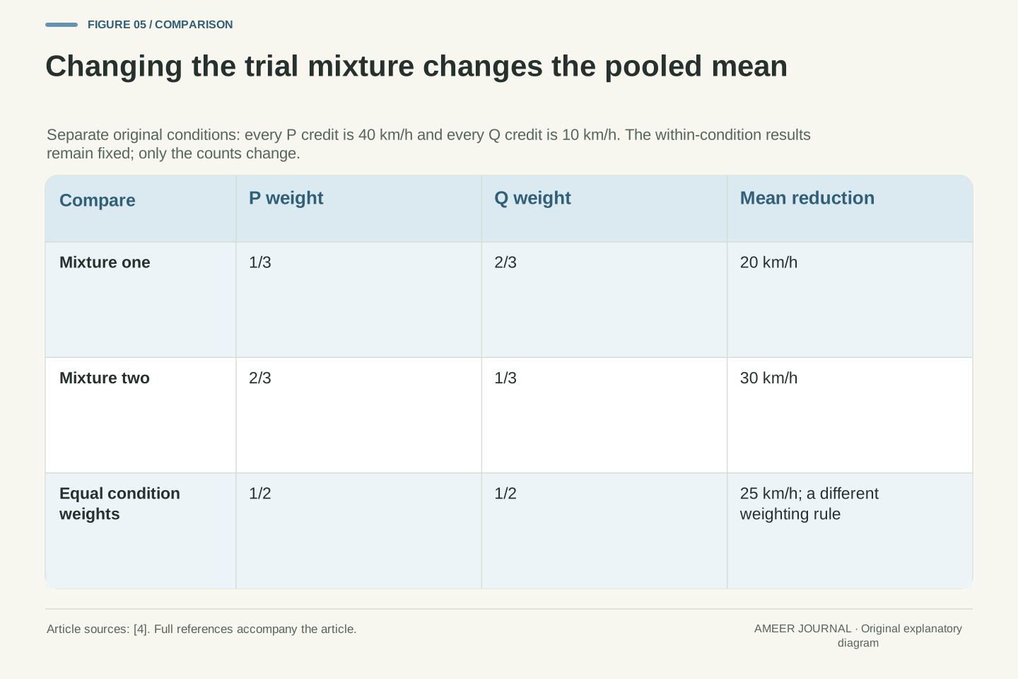
Now create two fictional conditions, P and Q, still using the 50-kilometre-per-hour reference. Each P record receives a credit of 40; each Q record receives 10. If there are two P records and four Q records, the total is 80 plus 40, or 120, across six rows. The pooled mean is 20. If there are four P records and two Q records, the total becomes 160 plus 20, or 180, and the pooled mean is 30. The reference and individual condition credits remain identical in the two mixtures.
Neither condition's assigned result improved. Only the mixture of records changed. Averaging the two condition means equally would instead give 25 in both cases. That is a different weighting choice, not an arithmetic correction to the pooled result. Frequency weighting follows the ordinary mean calculation. [4] When two reports use different mixtures, keep the condition results and their counts beside the total so that a changed sample composition is not silently described as better performance within a condition.
For constant within-condition means m_P=40 km/h and m_Q=10 km/h, the pooled trial mean is (n_P m_P+n_Q m_Q)/(n_P+n_Q). This is the frequency-weighted arithmetic mean. [4] Counts (2,4) give 20 km/h, while counts (4,2) give 30 km/h. The equally weighted condition mean, (m_P+m_Q)/2, remains 25 km/h. Both formulas are well-defined but summarize different observation weights. The pooled P/Q weights are 1/3 and 2/3 in the first mixture, then 2/3 and 1/3 in the second. Equal condition weights are 1/2 each.
This construction keeps every within-condition value fixed, so the changed pooled number cannot be attributed to an improvement inside P or Q. Nor does the equal-condition calculation automatically become the official or preferred score. Its appropriateness depends on the reporting question and specified method. Real comparisons should preserve the scenario identities, per-scenario results and weighting rule. A single pooled value cannot reveal whether its movement came from changed outcomes, changed composition or both.
A warning-only or absent result is not a measured zero
The IIHS explanation distinguishes some warning-only evaluations from the automatic-braking evaluations, and describes cases where higher-speed braking testing does not proceed after lower-speed results. [2] A field without a completed braking outcome must keep that meaning. It cannot automatically become a zero reduction, a successful avoidance or an additional ordinary trial. These alternatives would add a result that the record did not report.
For a separate paper example, suppose two observed credits are 40 and 50, while a third result is unknown. The observed-only mean is 45 across two rows. Filling the unknown with zero would produce 30 across three, but that would be an invented completed record. If the unknown is only known to lie between zero and 50, the complete three-row mean could lie anywhere from 30 to about 46.67. Keep both the missing status and the denominator visible instead of replacing uncertainty with a convenient number.
A warning-only evaluation and an unperformed braking evaluation are not observations of zero braking credit. The IIHS overview makes those distinctions within its scenario progression. [2] Consequently, a numerical dataset should retain a status field rather than coerce every absent reduction into a measured scalar. The warning field can contain evidence even when the braking field does not contain the result being averaged. A dash, a zero and an avoided label describe different records.
In the separate original record (40,50,unknown) km/h, the observed-only mean is 90/2=45 km/h. Under the additional bound 0≤unknown≤50 km/h, the complete mean ranges from 90/3=30 to 140/3≈46.6667 km/h. Setting the unknown to zero selects one endpoint without evidence. The observed-only mean also does not identify the complete mean; it names a different observation set. These deterministic possibilities require no assumption that missingness is random, and they supply no basis for substituting a population estimate.
An outcome record is not a real-world crash probability
Our A log's three avoided contacts out of six describe that invented list. They do not mean a car has a one-in-two chance of avoiding a collision on the road. We specified the rows ourselves and supplied no collection of real journeys, exposure counts or sampling method. Similarly, comparing speeds among the remaining contacts does not provide an injury calculation. The model contains no people, vehicle structures or collision mechanics with which to answer that different question.
The distinction does not make the numerical summaries useless. Each answers a precise question about a stated record: the amount credited, the number avoided, the spread, or the mean among contacts. Useful interpretation keeps those questions together without merging them. The particular vehicle's documentation also remains relevant to its functions and limitations, as NHTSA advises. [3] A reading exercise can clarify a report without becoming an instruction to try emergency intervention on a road.
The finite fraction k/n in our constructed logs is descriptive. It is not an estimator obtained from a specified sample of real-world collision opportunities. The original records have no exposure model, random selection mechanism or representative distribution of targets, speeds and conditions. A valid statement about their counts therefore must not be promoted into a crash-avoidance probability for a vehicle or user. More decimal places would not supply that absent sampling design.
The contact-only mean likewise describes a conditional subset, not an injury-severity model. Changing the avoidance count changes which cases remain in that subset, so conditional and all-record summaries can move differently. This is a property of the reporting sets, not an inconsistency requiring one statistic to be discarded. For an actual interpretation, the system's documented function and applicable report remain the evidence boundaries. [3] None of our calculations changes the driver's role, validates hardware or proposes a physical intervention test.
Keep the definition and the individual outcomes beside the average
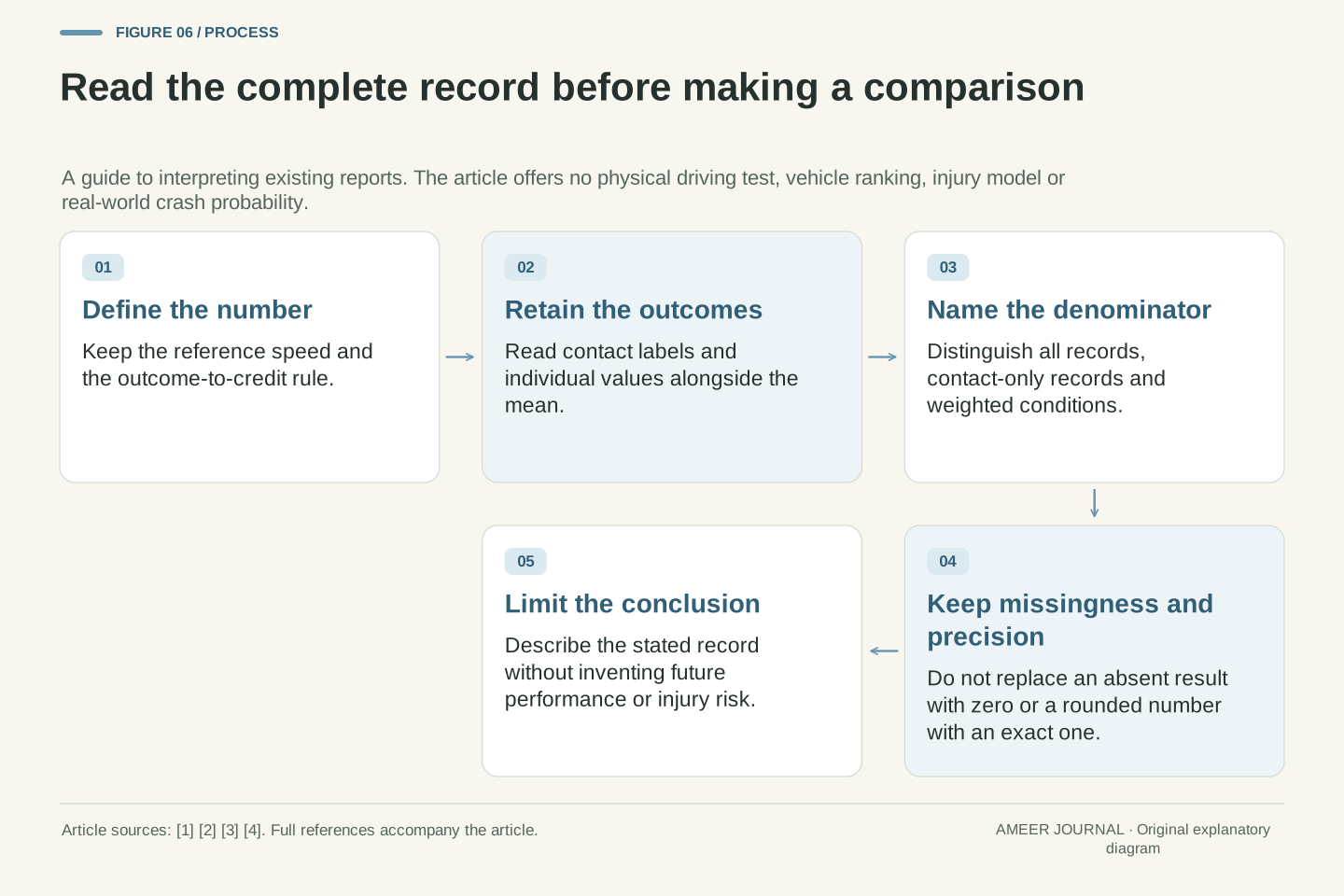
When reading a result, begin with its reference speed and the definition of reduction. Then look for the individual outcome labels and the number of records. Ask whether the stated mean includes every completed record, only contact cases, or an aggregation of several conditions. Retain the condition names and counts before combining them. Finally, check how the display rounds values and how it represents missing or warning-only results. These are questions about an existing report, not a request to conduct a test.
The original logs now make the reason clear. A and B share a mean reduction of 25, an all-record coded outcome mean of 25 and a median reduction of 25. They still have different avoided counts, contact-only means and ranges. No contradiction is hiding there: each number describes a different feature of the same complete record. A well-labelled explanation lets a reader see those features together instead of asking one headline average to count events it does not uniquely identify.
An interpretable result retains the reference definition, coding rule, outcome indicator, trial count, individual values, conditions, aggregation weights, missing-data statuses and displayed precision. These fields make it possible to reproduce a chosen statistic and determine what it omits. The source organizations distinguish functions and test outcomes; the original constructions show why the arithmetic must retain that distinction. [1][2][3][4] The necessary evidence is the actual reporting record and method, not a guessed universal conversion.
For the fixed-reference fixture, mean(v*)=V−mean(d) is recoverable, while the avoidance count generally is not. Adding a contact-only mean changes the conditioning set; adding a median still leaves our A/B ambiguity; rounding, unequal mixtures and missing rows introduce separate interpretation questions. Those are distinct, checkable limits. Keeping the complete rows and their definitions allows the average to do its intended job without turning it into an unsupported statement about every trial, a real vehicle's safety or future driving outcomes.
Sources & further reading
Explore the references behind this guide. External pages may change after our review.
- Vehicle-to-Vehicle Front Crash Prevention 2.0 Test Protocol — Version II, April 2025Insurance Institute for Highway Safety · Accessed 7 Nov 2026
- Front crash prevention: vehicle-to-vehicleInsurance Institute for Highway Safety · Accessed 7 Nov 2026
- Driver Assistance TechnologiesNational Highway Traffic Safety Administration · Accessed 7 Nov 2026
- Introductory Statistics 2e — Measures of the Center of the DataOpenStax, Rice University · Accessed 7 Nov 2026
Article updated 7 Nov 2026.
Found something we should revisit?
Good explanations get better with thoughtful feedback.