What you’ll take away
- A short record can use less total battery energy while using more energy per kilometre.
- A completed preparation allowance is separate from ongoing timed electricity and distance-dependent use.
- Actual preparation events matter; splitting a journey into more rows does not create new energy withdrawals.
- Two matching distance-energy points can identify a combined slope without identifying the heating power.
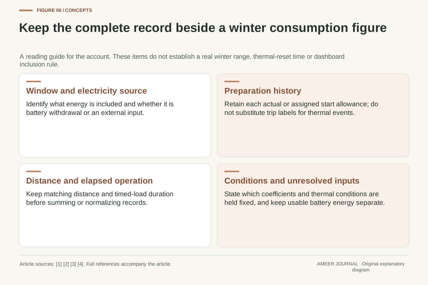
- Compare matching energy windows, thermal histories, durations and distances before interpreting a winter figure.
A higher figure per kilometre can accompany less total energy
A short winter journey can use less battery energy than a long journey while showing a larger number of watt-hours per kilometre. The two statements answer different questions: how much energy was used, and how that amount compares with the distance covered. Heating adds another layer because some preparation happens before moving, while other climate-control demand continues over time. Tesla’s support explanation identifies short trips and stops as situations in which climate control can run without corresponding vehicle movement. Argonne’s research account also distinguishes accessory demand from other cold-weather effects. [1][2]
We will use an original energy account to see how those ingredients interact. Every distance, duration, power and energy allowance below is invented. No vehicle was driven or tested. The account includes a completed preparation stage before departure, followed by a timed driving interval. That choice matters: it does not assume that every real short journey finishes warming its cabin or battery. Keeping the stages separate lets us ask why repeated cold departures, longer elapsed time and an unequal mix of journeys can produce different consumption figures.
Specific consumption is an energy-to-distance ratio, so a larger value does not by itself imply a larger total withdrawal. Winter operation makes the distinction useful because thermal demand need not scale directly with distance. Tesla describes climate operation during short trips and stops, while Argonne separates accessory loads, battery-energy availability and other temperature effects. [1][2] Those mechanisms motivate an account with distinct distance, elapsed-time and preparation terms rather than a single unexplained winter multiplier.
The following numerical records are original analytical constructions at a battery-withdrawal boundary. They are neither fitted vehicle data nor range predictions. Preparation is stipulated to be complete before the subsequent timed interval begins, and its whole assigned electrical energy is included. Consequently, the model does not describe an unfinished warm-up hidden inside a short driving interval. Fixed coefficients isolate accounting relationships; their constancy is an assumption to be examined before interpreting any real record.
Give preparation, driving distance and timed heating separate entries
Assign three amounts to our imaginary vehicle. Distance-dependent driving uses 0.15 kWh per kilometre. After preparation, a separate climate load draws 1.2 kW throughout the timed interval. Each explicitly declared cold preparation has already used 0.6 kWh before departure. At 30 kilometres per hour, every kilometre takes one-thirtieth of an hour, so ongoing heating adds 1.2 divided by 30, or 0.04 kWh per kilometre. The moving part therefore uses 0.19 kWh per kilometre before we add the preparation allowance.
All three entries are battery electricity, not heat delivered to a cabin. The timed 1.2-kW term starts after the separately counted preparation stage, avoiding double counting. DOE describes cabin and battery preparation before driving; SINTEF’s own research report separately discusses initial power, later power, duration and energy during preheating. [3][4] Those sources establish useful categories, not our numerical values. In particular, SINTEF’s reported grid-connected measurements cannot be silently relabelled as the battery-side amounts in this example.
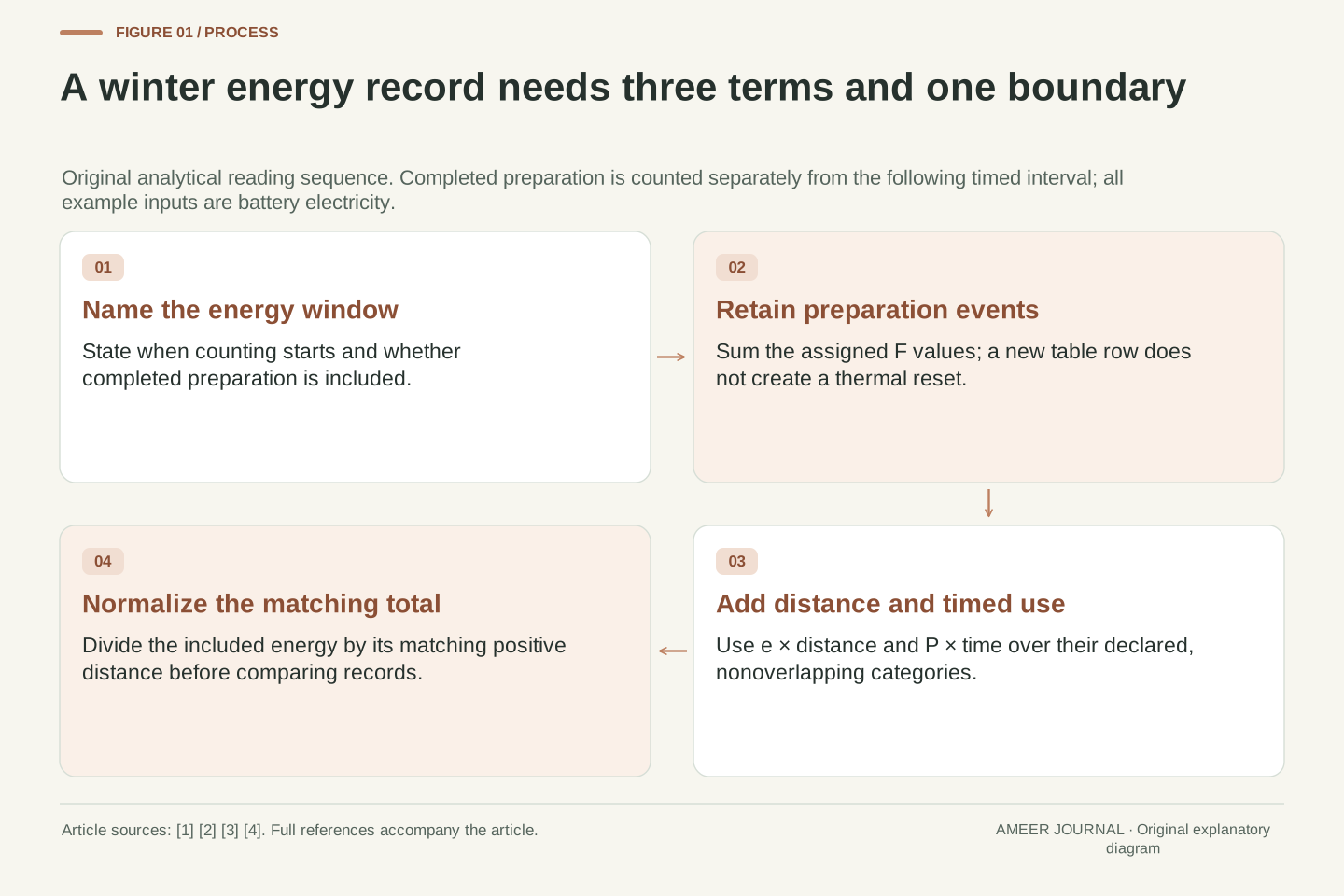
Define E=eD+PT+ΣF_j. Here e=0.15 kWh/km is the assigned distance-dependent coefficient, D is kilometres, P=1.2 kW is a separate constant post-preparation electrical load, T is its operating time in hours, and F_j are completed preparation withdrawals in kWh. A fully reset departure is assigned F_j=0.6 kWh. During uninterrupted motion at v=30 km/h, T=D/v and the combined moving coefficient is c=e+P/v=0.19 kWh/km. Each term therefore has a consistent electrical-energy unit.
The timed interval excludes the separately accounted preparation phase. F_j is not delivered thermal energy, a COP, a grid-meter reading or an assumed instantaneous heater pulse. It summarizes an already completed electrical withdrawal with no preparation duration assigned. DOE’s pre-driving-conditioning description and SINTEF’s institutional research report support separating stages and measurement boundaries. [3][4] The latter concerns mains-connected preheating; none of its empirical power or energy values supplies e, P or F_j here. Traction and other distance-dependent effects are already inside e rather than added again.
Compare a four-kilometre record with a sixteen-kilometre record
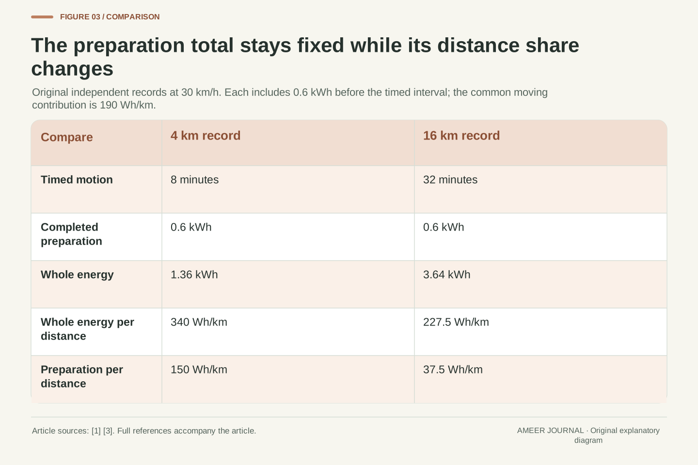
First consider a separately prepared four-kilometre journey. At the assigned speed, its driving time is eight minutes. Distance-dependent electricity is 0.15 times four, or 0.60 kWh. Timed heating uses 1.2 times eight-sixtieths of an hour, or 0.16 kWh. Add the completed 0.60-kWh preparation and the record totals 1.36 kWh. Dividing by four gives 0.34 kWh per kilometre, or 340 Wh/km. The preparation is a large part of this short record because all of it is included beside only four kilometres.
Now give a separate sixteen-kilometre journey the same preparation allowance and coefficients. Its thirty-two minutes of motion use 2.40 kWh for the distance term and 0.64 kWh for timed heating. Including preparation brings the total to 3.64 kWh, or 227.5 Wh/km. This longer journey uses more total electricity than the short one, yet less per kilometre. Neither number contradicts the other. The extra distance increases the moving-energy total while spreading the same initial allowance across a larger distance.
For D=4 km and T=4/30 h, the terms are eD=0.60 kWh, PT=0.16 kWh and F=0.60 kWh. Thus E_4=1.36 kWh and q_4=E_4/D=0.34 kWh/km=340 Wh/km. The eight-minute timed interval begins after preparation, so its short duration does not truncate the separately assigned F. This is essential to the construction: a real measurement beginning before an incomplete warm-up would require the actual energy accumulated within its own window. The equal 0.60-kWh distance and preparation terms are coincidental: one scales with distance and the other is assigned once.
For the independent D=16 km record, T=16/30 h, eD=2.40 kWh and PT=0.64 kWh. Adding the same F gives E_16=3.64 kWh and q_16=0.2275 kWh/km=227.5 Wh/km. Both records have the same post-preparation coefficient c=0.19 kWh/km. Their differing q values arise entirely from F/D under the specified model. Comparing E_16 with E_4 answers a total-energy question; comparing q_16 with q_4 answers a normalization question. The two comparisons need not have the same direction.
An initial allowance is diluted; it does not disappear
The preparation contribution alone is 0.6 divided by four, or 0.15 kWh per kilometre, in the short record. Over sixteen kilometres it becomes 0.0375 kWh per kilometre. Those are 150 and 37.5 Wh/km added to the same moving contribution of 190 Wh/km. The preparation electricity has not been recovered or cancelled. Its total stays at 0.6 kWh; only the distance used to describe that total has changed. This is why a low whole-trip average does not mean there was no energy cost at departure.
Imagine extending the four-kilometre record to sixteen kilometres without another preparation stage. The extra twelve kilometres use 12 times 0.19, or 2.28 kWh. They do not each inherit the original whole-record average of 340 Wh/km. That larger average included an allowance already paid once. Within this same account, making the preparation contribution no greater than 30 Wh/km requires at least twenty kilometres, because 600 Wh divided by twenty kilometres is 30 Wh/km. This is a relationship between quantities, not a reason to drive farther.
For positive D at fixed v and one preparation, q(D)=c+F/D. The preparation-specific contributions at 4 and 16 km are 0.15 and 0.0375 kWh/km. Their ratio is four because the denominators differ by four while F remains unchanged. The total E(D)=cD+F increases with D even as q(D) decreases toward c. No energy-recovery mechanism is involved; this is normalization of an unchanged additive term. For F>0, the derivative dq/dD=−F/D² is negative, and the decrease per additional kilometre becomes smaller as distance grows.
Under the same completed preparation, E(16)−E(4)=c(16−4)=2.28 kWh. The incremental consumption over that extension is 0.19 kWh/km, distinct from either whole-record ratio. Applying q_4 to every additional kilometre would repeatedly charge an initial allowance that the model assigns only once. The inequality F/D≤0.03 kWh/km gives D≥20 km for F=0.6 kWh, with equality at twenty. These conditional relationships do not establish an optimal journey length, a real thermal-reset time or the distance at which an actual vehicle reaches a steady temperature.
The number of cold preparations matters more than the number of table rows
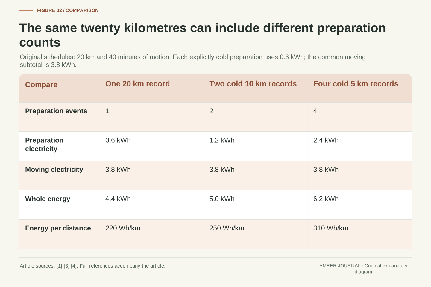
Keep total distance at twenty kilometres and total motion time at forty minutes. The common moving account is 3 kWh for distance plus 0.8 kWh for timed heating, or 3.8 kWh. One declared cold preparation brings the total to 4.4 kWh. Two separately cold ten-kilometre journeys have two allowances, making 5.0 kWh. Four separately cold five-kilometre journeys have four allowances, making 6.2 kWh. Their overall figures are therefore 220, 250 and 310 Wh/km despite equal total distance and motion time.
These are three different supplied schedules, not a prediction about what any particular stop will do. Their difference is the number of completed preparation events that the record explicitly includes. If someone merely divides the single twenty-kilometre journey into four spreadsheet rows, its energy remains 4.4 kWh. A formatting choice cannot create three additional heating events. To interpret a daily figure, keep the actual preparation history with the journey records instead of treating every new row, ignition event or destination as proof of a full cold reset.
For equal D=20 km and T=2/3 h, eD+PT=3.8 kWh. With N identical, fully assigned preparations, E_N=3.8+0.6N kWh. The independent N=1, 2 and 4 schedules yield 4.4, 5.0 and 6.2 kWh, respectively, or 220, 250 and 310 Wh/km over twenty kilometres. N counts the stipulated energy events; it is not inferred from the number of destinations. The model holds total timed operation and the distance coefficient fixed while varying that count. Each added 0.6-kWh event contributes 30 Wh/km to this fixed twenty-kilometre aggregate.
Additivity also provides an invariance check. Subdivide the one-preparation record into any number of nonoverlapping distance/time rows, assign its single F to exactly one row, and the sum remains eΣD_i+PΣT_i+F=4.4 kWh. Assigning F to every bookkeeping row would change the physical model rather than improve its resolution. Conversely, merging four genuinely separate preparation records into one daily row does not remove their four allowances. Aggregation should preserve events, included time and energy, even when the number of displayed rows changes.
A stop does not tell you how much preparation comes next
A vehicle can stop without its next thermal condition being specified. A label such as second trip does not tell us the cabin temperature, battery temperature, elapsed parking time or climate-control history. Tesla describes ongoing temperature regulation and loads while parked, while SINTEF identifies starting conditions and duration among the variables in its research account. [1][3] That is why our fixed 0.6-kWh allowance belongs only to departures explicitly assigned that amount. It should not be attached automatically to every interruption in movement.
For a separate two-journey case, keep twenty kilometres and forty minutes of timed motion, but supply preparation amounts of 0.60 and 0.15 kWh. The moving subtotal remains 3.8 kWh; the preparation subtotal is now 0.75, giving 4.55 kWh overall. We have not calculated a cooling curve that produces the second amount. It is new information supplied to the account. The difference from the two-full-preparation total of 5.0 kWh is 0.45 kWh, showing precisely which changed input caused the result.
The general expression uses ΣF_j because the individual preparation withdrawals need not be identical. A chronological stop count cannot establish those values. Actual thermal state and energy use depend on vehicle and operating history; the manufacturer and SINTEF descriptions identify relevant variation without providing a universal reset rule. [1][3] The model therefore distinguishes N identical assigned allowances from a general sequence of separately supplied F_j values.
For the independent case F_1=0.60 kWh and F_2=0.15 kWh, with D=20 km and T=2/3 h unchanged, E=3.8+0.75=4.55 kWh. Relative to two full 0.60-kWh allowances, the reduction is exactly 0.45 kWh. It is not a derived residual-heat fraction, a temperature estimate or evidence that a particular parking duration saves that amount. If the second withdrawal were unknown, the total would remain conditional on it. Replacing missing preparation information with either zero or a full allowance would add an unstated assumption.
The same distance can contain a different heating duration
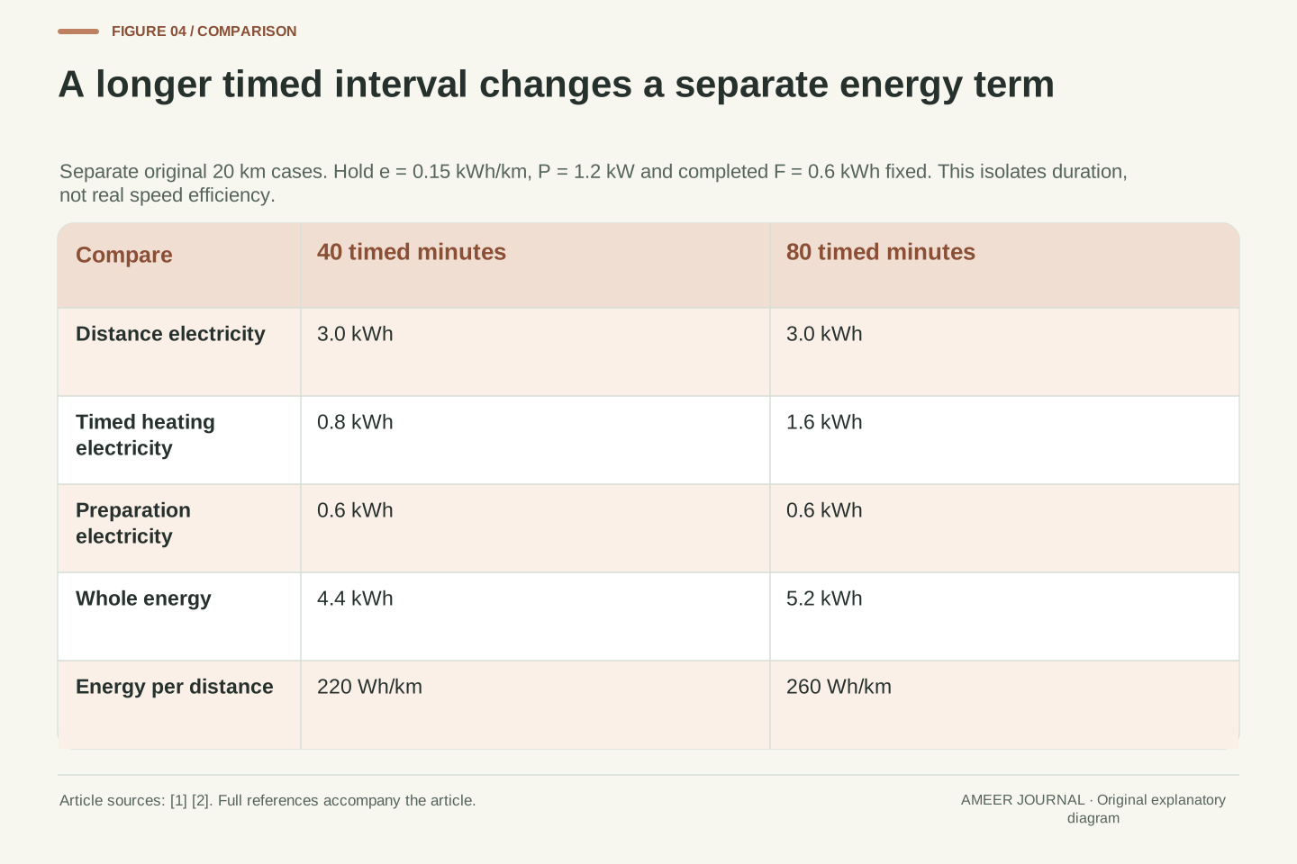
Return to one preparation and twenty kilometres. At forty minutes of timed operation, the 1.2-kW load uses 0.8 kWh. If that interval instead lasts eighty minutes while the same load continues, it uses 1.6 kWh. Keeping the distance-dependent term at 3 kWh and preparation at 0.6 gives totals of 4.4 and 5.2 kWh. The corresponding whole-record figures are 220 and 260 Wh/km. Distance stayed equal; the time-dependent part doubled. No second preparation was added.
This comparison deliberately holds the driving coefficient fixed. It is not a claim that driving at half the speed always increases an EV’s total electricity use. Actual speed, road conditions and thermal operation can change several inputs together. [1][2] The calculation isolates one question: what happens if the included 1.2-kW load operates for forty additional minutes? It adds 0.8 kWh. A distance-only record cannot establish that duration, and a preparation-only explanation would miss it entirely.
For D=20 km, F=0.6 kWh and e=0.15 kWh/km, changing T from 2/3 h to 4/3 h changes PT from 0.8 to 1.6 kWh. The totals are E_a=4.4 kWh and E_b=5.2 kWh, giving q_a=0.22 and q_b=0.26 kWh/km. The difference is PΔT=0.8 kWh. It is independent of the fixed preparation term in this particular sensitivity comparison. Dividing that difference by the unchanged twenty kilometres gives 0.04 kWh/km. This increment comes from the added operating time, while the initial allowance remains counted only once.
Attributing the difference to a real speed change would require a broader model: aerodynamic, rolling, propulsion and thermal loads can change with conditions. The retrieved manufacturer and laboratory accounts describe several such influences. [1][2] Here e, P and F are held constant by construction. The longer interval can be interpreted only as an assigned operating-time change within that boundary. It does not prescribe a driving speed, predict a traffic queue’s energy use or justify reducing a climate function needed for visibility or comfort.
A daily average must preserve the energy in both journeys
Combine the original four-kilometre and sixteen-kilometre records, each with its own complete preparation. Their energies add to 1.36 plus 3.64, or 5.0 kWh; their distances add to twenty kilometres. The combined figure is therefore 250 Wh/km. It lies between 340 and 227.5, but it is closer to the longer journey’s figure because that journey supplies four-fifths of the distance. The shorter record contains a whole preparation allowance, yet it does not represent half the kilometres simply because it occupies one line.
The unweighted average of the two figures would be 283.75 Wh/km. Multiplying that by the actual twenty kilometres would invent 5.675 kWh, which does not match the supplied 5.0-kWh total. Weighting by distance repairs the mismatch. This is especially useful when comparing daily records with different mixes of short and long cold journeys. Keep the preparation energy inside whichever records include it, then add matching energy and distance totals before comparing the aggregate.
The aggregate is q_bar=(E_4+E_16)/(4+16)=5/20=0.25 kWh/km. Equivalently, distance weights 1/5 and 4/5 give (1/5)(0.34)+(4/5)(0.2275)=0.25 kWh/km. The two preparations remain present in the numerator. This agrees with the N=2 twenty-kilometre account because e, P, total timed duration and total preparation energy also match. The result can also be recovered as c+2F/(20 km)=0.19+0.06=0.25 kWh/km, connecting the combined figure directly to the two preparation events.
By contrast, the unweighted mean is (0.34+0.2275)/2=0.28375 kWh/km. Applying it to twenty kilometres gives 5.675 kWh, an excess of 0.675 kWh over the constructed record. Equal record weights implicitly replace the actual distance weighting. This is an accounting mismatch, not evidence of a different heater efficiency. A comparison across days should first preserve the same included loads and event boundaries, then ask whether different distances, preparation counts or operating times explain the resulting aggregate.
Two supplied points can identify a combined slope and an allowance
The four- and sixteen-kilometre examples can also be read in reverse. Their energy difference is 3.64 minus 1.36, or 2.28 kWh. Their distance difference is twelve kilometres. Dividing gives 0.19 kWh per additional kilometre. Under our declared straight-line account, that is the moving contribution. Subtract four times 0.19 from the short record’s 1.36 kWh and 0.60 kWh remains as the preparation allowance. Putting those two values back into both original records reproduces their supplied energy totals.
This reverse calculation works because the two original records were deliberately built with the same preparation amount, speed and constant moving coefficient. A pair of real trip readings does not establish those conditions merely by having different distances. Measurement boundaries could differ, heating could change or the vehicle might start in different thermal states. The useful result is narrower: within the supplied model, the two points determine a slope and an intercept. They have not yet revealed how much of that slope belongs to the distance term and how much belongs to timed heating.
At fixed v=30 km/h and a common F, the model is affine: E(D)=cD+F, where c=e+P/v. From the two exact constructed points, c=(3.64−1.36) kWh/(16−4) km=0.19 kWh/km, and F=1.36 kWh−(0.19 kWh/km)(4 km)=0.60 kWh. Both units and the common-condition assumptions matter. The inferred intercept is the stipulated completed preparation allowance, not an independently measured thermal quantity. Substitution recovers 0.19×4+0.60=1.36 kWh and 0.19×16+0.60=3.64 kWh, with the distances in kilometres and slope in kWh/km.
Two distinct distances identify c and F only within this specified affine family. They do not prove that the family describes real observations, establish constant coefficients or determine a physical cause. No noise model, uncertainty interval or regression claim is supplied. In particular, c combines two parameters at the fixed speed: distance-dependent consumption and timed electrical power divided by speed. The next comparison constructs two different parameter sets with the same c, demonstrating an ambiguity that exact arithmetic alone cannot remove.
The same two trip totals can conceal different heating powers
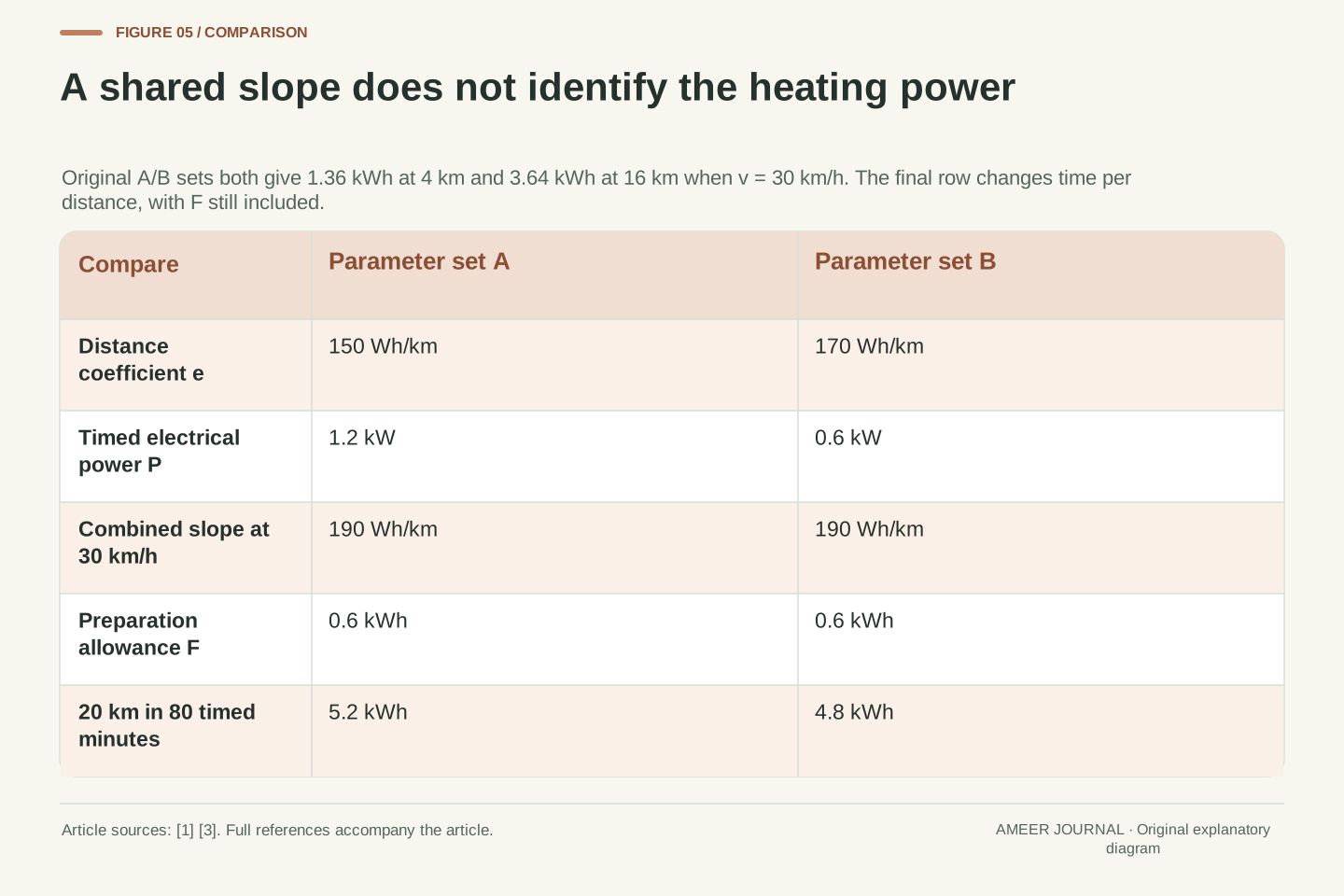
Our first parameter set uses 0.15 kWh per kilometre for distance and 1.2 kW for timed heating. At thirty kilometres per hour, the heating contribution is 0.04 kWh per kilometre, giving 0.19 in total. Now invent a second set: 0.17 kWh per kilometre for distance and 0.6 kW for timed heating. Its heating contribution is 0.02 kWh per kilometre, again giving 0.19. With the same 0.6-kWh preparation, both sets reproduce the four- and sixteen-kilometre energy totals exactly.
A separately supplied twenty-kilometre, eighty-minute record would distinguish them within this model. The first set gives 3.0 plus 1.6 plus 0.6, or 5.2 kWh. The second gives 3.4 plus 0.8 plus 0.6, or 4.8 kWh. Different durations separate the time-dependent contribution from the distance-dependent contribution when the coefficients really remain fixed. We are comparing declared mathematical records, not asking someone to perform a road test. Agreement with two totals does not uniquely identify the heater’s electrical power.
Parameterization A is (e_A,P_A)=(0.15 kWh/km,1.2 kW). Parameterization B is (e_B,P_B)=(0.17 kWh/km,0.6 kW). At v=30 km/h, both yield c=0.19 kWh/km. With the same F=0.6 kWh, their predictions agree for every positive distance at that fixed speed, including the two original points. This is a structural non-identifiability in the chosen data arrangement, not a rounding artifact or a claim about actual vehicle instrumentation. At the fixed speed, T=D/v makes the time input proportional to the distance input, so the two components cannot vary independently across those records.
At D=20 km and T=4/3 h, A gives 5.2 kWh while B gives 4.8 kWh. The changed time-to-distance relationship breaks their previous equality under the fixed-parameter assumption. An independent observation at such a different relationship could constrain the partition in this ideal model; real inference would also require matching thermal history, boundaries and uncertainty. No observed third record is claimed. The counterexample establishes why a well-matched total-consumption curve need not uniquely determine the underlying distance and timed-load components.
Changing the record window changes which energy is included
Our four-kilometre record includes preparation, so it totals 1.36 kWh and 340 Wh/km. A different window beginning immediately after that preparation includes only 0.60 kWh for distance plus 0.16 kWh for timed heating. Its total is 0.76 kWh, or 190 Wh/km. These are two descriptions of explicitly different observation windows around the same constructed journey. The smaller figure does not mean the earlier 0.60-kWh withdrawal vanished; it lies outside the second window.
That is a useful question to bring to a trip display or research table: when did the energy account start, and which loads does it include? Tesla describes driving and parked-energy categories, while SINTEF’s report explicitly discusses electricity used for preheating from the mains. [1][3] Their categories should not be assumed to match every dashboard or our battery-side account. Before comparing figures, match the source of electricity and the window as well as the distance. Otherwise, an apparent improvement may be a changed inclusion rule.
For the four-kilometre construction, E_full=F+eD+PT=1.36 kWh, while E_after=eD+PT=0.76 kWh. Their normalized values are 0.34 and 0.19 kWh/km, respectively. The difference is exactly F/D=0.15 kWh/km. Both calculations are internally correct because they explicitly name different observation windows. Treating them as interchangeable measurements of one unchanged window would be incorrect. Appending the preparation interval to the after-departure record restores E_full exactly without changing the four-kilometre distance denominator.
The sources establish that driving, parked and preheating accounts can be distinguished, and that grid-connected research measures a different input boundary from battery withdrawal. [1][3] They do not establish a universal dashboard inclusion rule or guarantee that a connected vehicle draws all conditioning energy from one source. If external electricity, charging losses or a different starting event is introduced, the account must be extended accordingly. The original F is included battery energy; merely moving its row outside a displayed interval does not eliminate it from a wider energy total.
Read the thermal history, the clock and the distance together
A useful winter-consumption record answers several concrete questions. Does its energy include preparation before moving? How many preparations actually occurred, and were their amounts supplied or assumed? How long did timed loads operate? What total distance accompanies that same energy? Finally, were the starting condition and the intended cabin service comparable? Those details let you distinguish a short-distance effect from a longer heating period or a different preparation history. A single Wh/km figure cannot supply all of them.
Keep available battery energy separate from consumption too. Argonne’s research account identifies temperature effects on usable energy as well as accessory demand. [2] Our arithmetic has held the consumption coefficients and event allowances fixed; it has not calculated how much energy a real pack can provide in the cold. The practical reading skill is to preserve the full account before extrapolating. A high short-trip figure may be perfectly consistent with its included startup energy and distance, while still being a poor description of a differently timed or differently prepared journey.
A reproducible account retains D, T, the preparation sequence F_j, the electrical boundary and the observation window. It also states whether e and P are fixed assumptions, measured interval summaries or unresolved quantities. The examples show distinct changes: additional preparation events, altered duration, changed distance weighting and changed inclusion windows. Each changes a specific part of E=eD+PT+ΣF_j, so the explanation should identify that part rather than use a generic cold-weather multiplier.
The laboratory account separately identifies temperature-related usable-energy effects. [2] That numerator for a range calculation is outside the present consumption construction. No full-pack distance follows without additional assumptions about available energy and future operation. Likewise, the reverse fit identifies only what the supplied records constrain; it does not turn a constant allowance into a physical law. Read the thermal history, clock and distance together, and keep the distinction between an exact conditional account and a real vehicle’s changing operating state.
Sources & further reading
Explore the references behind this guide. External pages may change after our review.
- Range Tips | Tesla SupportTesla · Accessed 7 Nov 2026
- Passenger Car BEVs under Extreme Weather -
Vehicle & Mobility Systems Department - Argonne National LaboratoryArgonne National Laboratory · Accessed 7 Nov 2026
- What’s the best way of warming up your electric car? - SINTEFSINTEF · Accessed 7 Nov 2026
- Winterizing Your Electric Vehicle | Department of EnergyU.S. Department of Energy · Accessed 7 Nov 2026
Article updated 7 Nov 2026.
Found something we should revisit?
Good explanations get better with thoughtful feedback.