What you’ll take away
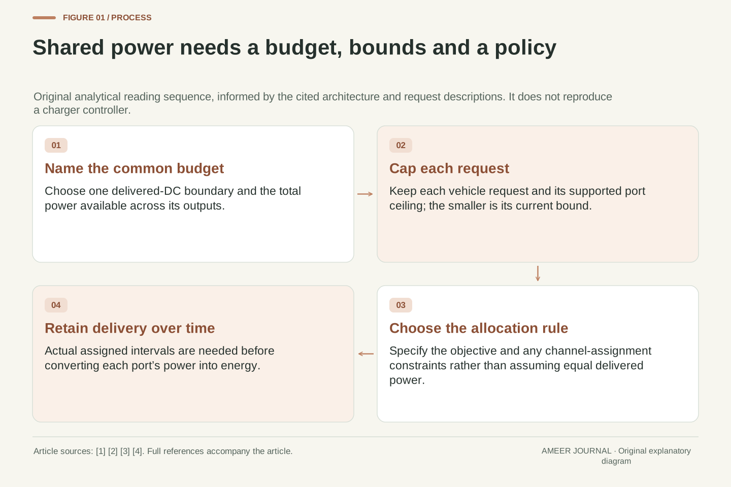
- A common DC-output budget couples otherwise distinct vehicle ports.
- With capped requests of 90, 80 and 20 kW, original progressive filling shares a 150 kW budget as 65, 65 and 20 kW.
- Priority, proportional and max-min rules can obey the same bounds while delivering different shares.
- Whole channel assignments constrain capacity; they do not require every assigned channel to deliver its full rating.
- A power allocation needs a time history before it determines per-vehicle delivered energy.
A rating beside one cable does not describe the shared supply
Three vehicles can be connected to three charging ports without having three independent supplies behind them. Some DC charging systems distribute power from a common cabinet to separate dispensers. ChargePoint's retrieved Power Block introduction describes that division of roles, while a June 2023 Kempower explanation describes centralized power distributed among charging outputs. [1][2] The number beside an individual cable therefore needs another fact: how much power the shared system can provide to all connected vehicles together.
This article builds an original three-vehicle example to explain that shared limit. Every request, rating, allocation and duration in the calculation is invented; no charging station or vehicle was tested. We first allow power to be divided continuously, then introduce a separate system with whole assignable converter channels. The second model reveals why a total power figure can still miss an allocation constraint. Along the way, we keep the equipment ceiling, the vehicle's request, the chosen policy and the resulting delivered power as separate entries.
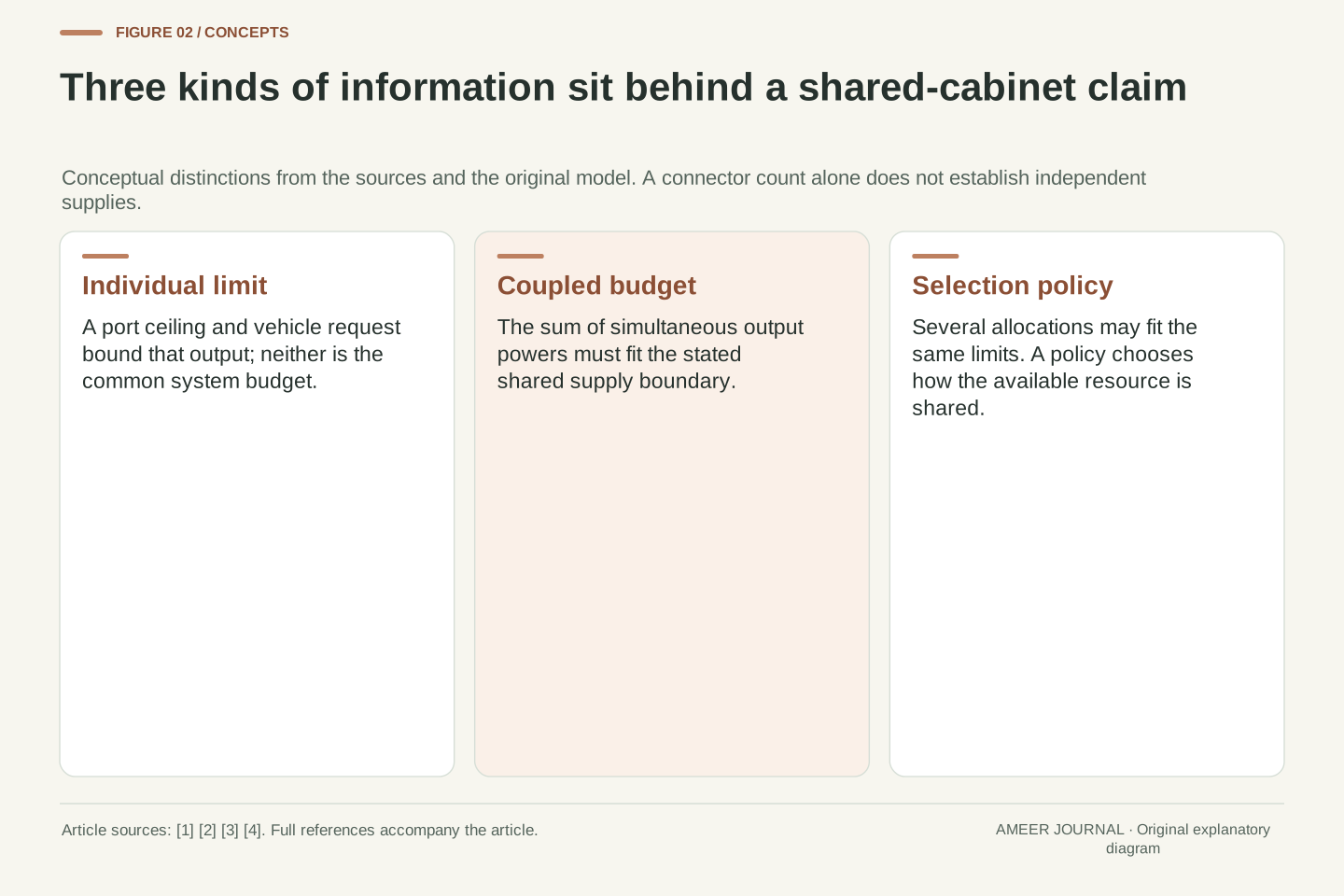
A set of per-port ratings does not specify the feasible simultaneous output vector of a shared charging system. The retrieved ChargePoint architecture separates cabinet conversion and DC distribution from downstream dispensers. Kempower's dated description likewise distinguishes a centralized supply and dynamically shared outputs. [1][2] Coupled limits arise because several outputs can draw on a common resource. Summing individual maxima can therefore describe an operating point the aggregate supply cannot support.
The original analytical models below use one common DC-output boundary and stipulated compatible sessions. They separate request and port caps, an aggregate budget, an allocation objective and, later, assignable channel capacity. Supported voltage/current envelopes, communication, thermal conditions and ideal output tracking are assumptions, not conclusions of the arithmetic. No proprietary controller is reproduced. The continuous and discrete examples deliberately have different feasible sets; their comparison shows why a policy name and a total wattage are insufficient to reconstruct what a real charging site will deliver.
Count ports separately from converters and connectors
The Alternative Fuels Data Center distinguishes a station location, a charging port and a connector. Its port definition serves one vehicle at a time, even if that port offers more than one connector. [3] A location can contain several ports, and a dispenser can be one visible part of a larger arrangement. Counting plugs is therefore not enough to establish simultaneous vehicle capacity, and counting simultaneous ports is not enough to establish independent power supplies.
ChargePoint's retrieved guide places power conversion and distribution in a cabinet, with downstream equipment receiving its output. It also emphasizes that the actual system architecture varies with configuration. [2] Our model starts after that architectural question has been settled: three distinct vehicle ports share one stated DC-output budget. That budget is not an upstream utility-meter reading. Conversion losses and cabinet auxiliaries would need separate treatment before translating an AC site limit into this DC quantity. All comparisons below stay at the same boundary.
Use AFDC's terminology: a location may contain multiple ports, while one port supplies one vehicle at a time despite possible alternative connectors. [3] This is a count of simultaneous vehicle interfaces, not a count of isolated upstream sources. ChargePoint's introduction separately identifies cabinet conversion, DC distribution and dispenser input paths, and qualifies its illustrated architecture as one possible configuration. [2] These distinctions prevent a visible cable count from becoming an unsupported power-capacity calculation.
Define p_A, p_B and p_C as delivered DC powers at the three vehicle interfaces. The common budget B bounds their sum at that same accounting boundary. It is not automatically equal to an AC supply rating or a cabinet's gross internal rating. We stipulate that upstream conversion and auxiliary effects have already been excluded from B. Consequently, unused budget later means available output capacity that was not allocated or drawn, not energy dissipated as heat. A different physical boundary would require an additional balance before comparing the numbers.
Give the shared budget and every vehicle its own limit
Assign port ceilings of 120, 100 and 80 kilowatts to A, B and C. Their present requests are 90, 80 and 20 kilowatts. The shared DC-output budget is 150 kilowatts. The three port labels add to 300, but that does not double the available common supply. Even the requests add to 190, which is more than the system can deliver at once. Some requests must therefore be served below their present maximum if all three remain in this shared arrangement. At least 40 kilowatts of their combined request cannot be served at that instant.
For each vehicle, first take the smaller of its request and its port ceiling. The resulting limits are 90, 80 and 20 kilowatts. The manufacturer explanation of DC charging describes continuing communication and changes in requested power; it does not make an equipment rating a command to consume that rating. [4] We assume these three numerical limits are supported for the present operating point. The next question is how to choose a delivered value below each limit while keeping their sum within 150.
Let c=(120,100,80) kW be port ceilings and r=(90,80,20) kW be requests. Define u_i=min(c_i,r_i), so u=(90,80,20) kW. With B=150 kW, the continuous feasible set is 0≤p_i≤u_i and p_A+p_B+p_C≤B. The sum of the port ceilings is 300 kW and the sum of capped requests is 190 kW; neither replaces the shared 150 kW constraint. The original values describe one supported operating point rather than an entire voltage/current envelope. They leave at least 40 kW of the combined request unserved.
The vehicle-request distinction is consistent with ChargePoint's description of ongoing vehicle communication and changing requested power. [4] We do not infer why a particular request is lower, or guarantee that a real station tracks it exactly. For the mathematical examples, a chosen feasible allocation is stipulated to be delivered. These constraints identify permissible vectors but do not select one vector. A policy or objective must supply that missing information, and different choices can obey the same physical and request limits.
Equal quotas can leave some of the budget unused
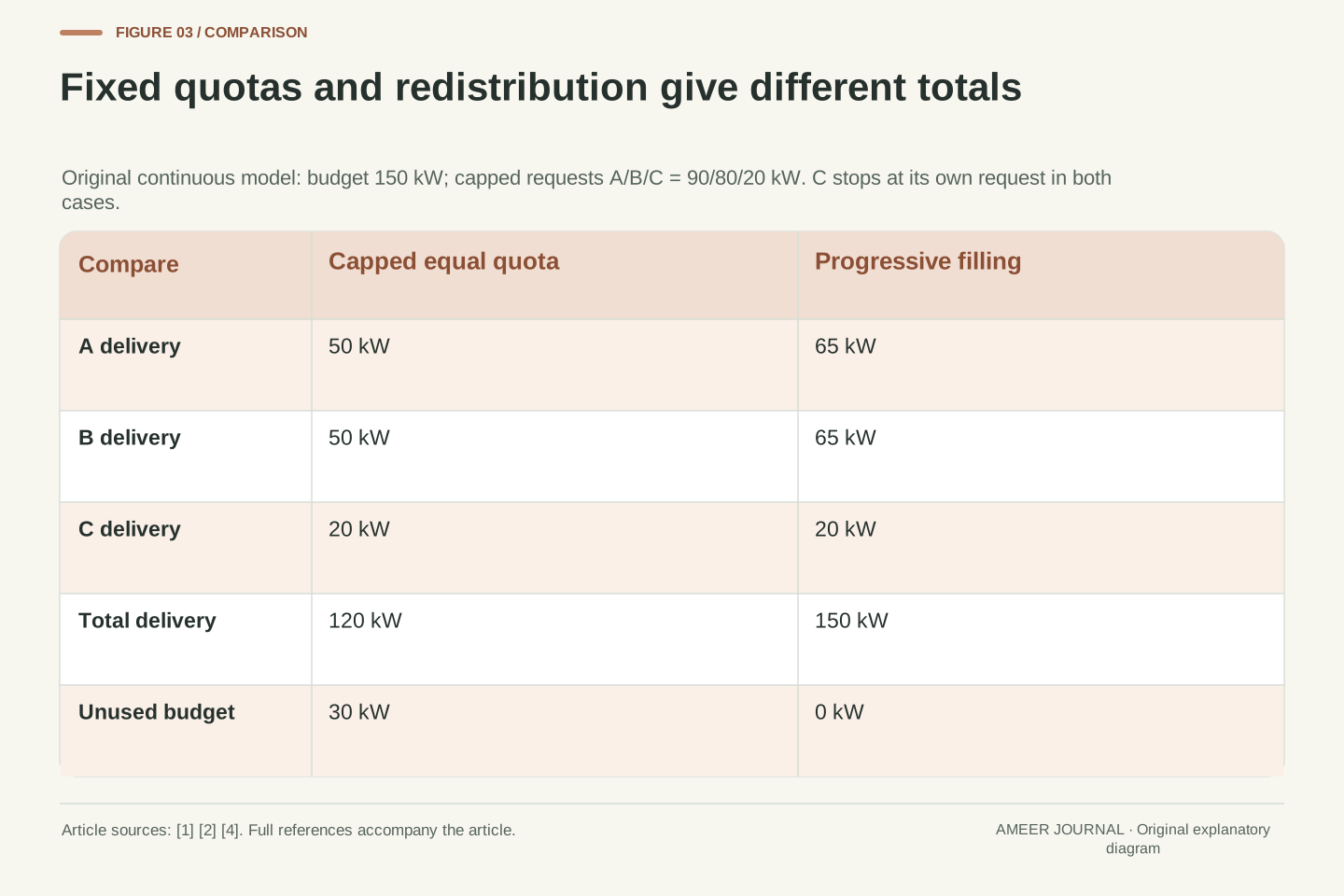
A first attempt divides 150 equally across three ports, giving a quota of 50 kilowatts each. A and B can use their quotas. C requests only 20, so this capped-quota rule delivers 50, 50 and 20. The total is 120 kilowatts, leaving 30 of the common budget unused. Giving C all 50 would violate its stated request limit; the spare capacity cannot be converted into a demand merely by writing an equal number in every column. Only A and B still have unsatisfied demand.
Nothing in the budget alone says where the unused 30 should go. Keeping fixed quotas is one possible mathematical choice, although our next policy will redistribute the remainder. The distinction is between a share initially offered and the value actually used under the bounds. It also prevents a misleading efficiency statement: the unused 30 kilowatts are not a measured electrical loss. In this example they were never delivered, and no input-energy or heat account has been supplied.
Under an equal-quota rule, set q=B/3=50 kW and p_i=min(u_i,q). The resulting vector is (50,50,20) kW, with total 120 kW. Residual budget is B−Σp_i=30 kW. This rule satisfies every constraint but does not maximize total output for the continuous feasible set. The unused quota at C does not automatically modify the assignments at A and B; that requires an additional redistribution rule. Unsatisfied capped demands are 40, 30 and 0 kW, totalling 70 kW; they are distinct from the 30 kW of cabinet headroom.
This example distinguishes feasibility from an objective. A feasible allocation can leave headroom even when other requests remain unsatisfied. It also distinguishes offered capacity from actual delivery: forcing p_C=50 kW would exceed u_C=20 kW and leave the defined model. Calling the residual a conversion loss would cross another boundary incorrectly. We have specified no AC input or dissipation, only an output budget. The next policy uses that remaining feasible headroom while respecting the same capped requests.
Raise uncapped shares together until the budget is used
Imagine raising all three delivered shares together from zero. Once each reaches 20 kilowatts, C has all it requests and stops increasing. A and B can continue rising together. After assigning C its 20, the remaining 130 divides equally between A and B, giving 65 each. The final allocation is therefore 65, 65 and 20 kilowatts. It uses the full 150 without exceeding any request or port ceiling. A still requests 25 more and B requests 15 more, but no common budget remains.
This is an original progressive-filling rule: hold a vehicle at its own limit once it reaches that limit, then share the remainder among those still able to increase. It aims to raise the smallest feasible delivered shares first. It does not promise equal percentages of each vehicle's request, and it is not a reconstruction of a manufacturer's named mode. A and B receive equal power here because neither reaches its cap before the remaining common budget runs out.
For the continuous model, use capped progressive filling, equivalently a max-min allocation. Choose a common level λ and set p_i=min(u_i,λ), with Σp_i=min(B,Σu_i). At B=150 kW, C saturates at 20 kW and 2λ+20=150 gives λ=65 kW. Since 65 is below both remaining caps of 90 and 80, the vector (65,65,20) is feasible and exhausts the available budget. If all demands were met first, additional budget would remain unused. Here, unserved request totals 40 kW while budget headroom is zero.
The max-min objective concerns delivered power: after a capped smaller request is satisfied, it raises the next-smallest shares as far as possible. It is different from equalizing p_i/u_i or preserving arrival priority. Manufacturer descriptions establish that alternative policy concepts exist, but the equation above is our expressly stipulated rule. A product's label alone does not establish its exact rounding, channel assignment, response time or treatment of minimum-power sessions. Those implementation details remain outside this continuous model.
The same limits allow several different allocations
Now keep every limit unchanged but give A priority, then B, then C. A receives its requested 90 kilowatts; the remaining 60 go to B; C receives zero during this assigned interval. That uses the same 150-kilowatt budget as progressive filling, yet the experience at the three ports is very different. Kempower's dated explanation describes both shared and arrival-priority concepts. [1] Our numerical priority rule is a separate paper policy, not a claim that its hardware produces these particular values.
Another original rule gives every vehicle the same fraction of its capped request. Since 150 divided by 190 is fifteen nineteenth parts, the allocations are about 71.05, 63.16 and 15.79 kilowatts. Again, their exact total is 150. This rule gives C less than its full request even though progressive filling satisfies C. Neither total output nor the number of connected vehicles identifies which policy was used. The objective must be named before calling one distribution better for a particular purpose.
Under a stipulated strict A-then-B-then-C priority rule, sequentially allocate min(request cap, remaining budget). This yields (90,60,0) kW. Under a proportional rule p_i=u_iB/Σu_i, the exact vector is (1350/19,1200/19,300/19) kW, whose sum is 150 kW. Both are feasible, as is the progressive-filling vector, but they optimize or preserve different relationships. Zero allocation in the priority example means no delivered power at C during that interval, not an additional waiting-time model.
Kempower's June 2023 description provides bounded context for different sharing and priority choices. [1] It is not evidence that either original mathematical rule reproduces a current implementation. Max-min power sharing, equal fractional satisfaction and arrival priority are different objectives; aggregate throughput alone cannot choose among them. Rounded proportional values are display approximations, so use the exact fractions when checking their sum. These comparisons make the policy an explicit input instead of hiding it inside a headline cabinet rating.
A change at one vehicle can change another vehicle’s share
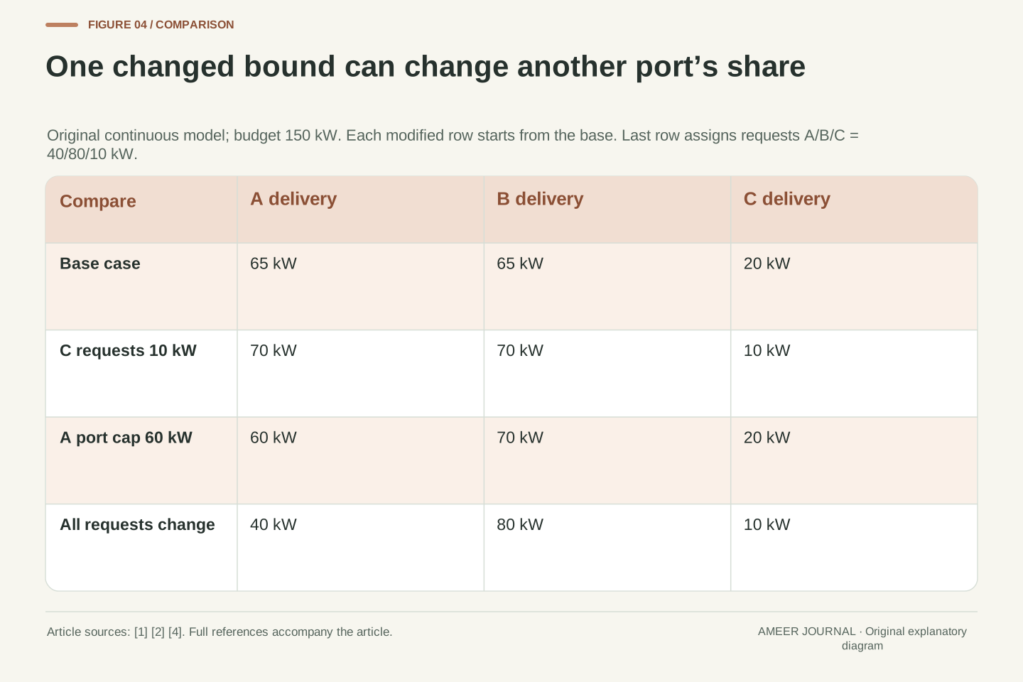
Return to continuous progressive filling and the 150-kilowatt budget. If only C's request falls from 20 to 10, A and B each rise from 65 to 70. Their own requests did not change; more of the shared budget became available to them. In a separate case, restore the original requests but lower A's supported port ceiling to 60. The allocation becomes 60, 70 and 20. A's local constraint now releases capacity that B can use. B gains five kilowatts in both cases, for different reasons.
For a third, separate case, assign requests of 40, 80 and 10. Their total is only 130, so all three requests can be met and 20 of the 150 remains unused. There is no unsatisfied request within this model to receive it. Real vehicle requests can vary during charging, as the manufacturer explanation describes. [4] These assigned changes establish no particular cause, battery temperature or state of charge. They show why an unchanged cabinet and cable can accompany a changing delivered share.
With B=150 kW, changing only C's request to 10 gives u=(90,80,10) kW. Progressive filling solves 2λ+10=150, so p=(70,70,10) kW. Separately, restoring the original requests and changing only A's port cap to 60 gives u=(60,80,20), hence p=(60,70,20) kW. In each case one changed bound alters another port's allocation through the common budget; the changes are not applied cumulatively. C has reached its 10 kW request in the first case, while A’s 60 kW port ceiling binds in the second.
A third request vector (40,80,10) kW totals 130 kW, below B. All requests are met and 20 kW remains unused. That residual has a different reason from the fixed-quota residual: no additional demand is available in the present model. ChargePoint describes changing vehicle communication and requests during charging. [4] We use that qualitative context without deriving a physical charging curve or interpreting a lower observed value as a fault. A measured power alone does not reveal which request, port, group or policy constraint selected it.
More common power helps only the requests that remain unsatisfied
Keep the original requests of 90, 80 and 20 and increase only the common budget. At a budget of 60, all three can receive 20. From there, C stays at its request while A and B rise together. A budget of 180 gives 80, 80 and 20. B then reaches its request too, so increasing the budget to 185 gives the extra five only to A: 85, 80 and 20. C’s unchanged twenty-kilowatt request is already fulfilled throughout these increases. It gains nothing from extra capacity assigned elsewhere.
At a budget of 190, every original request is satisfied: 90, 80 and 20. Raising the budget again to 200 changes none of those deliveries, leaving ten unused. That result does not prove that additional capacity could never help other sessions. It says that these particular requests are already met under this rule. A cabinet rating must therefore be interpreted with the connected demand and allocation policy, rather than assumed to produce a proportional increase at every port whenever it increases.
For fixed u=(90,80,20) kW, progressive filling has three active budget regions. For 0≤B≤60 kW, every share is B/3. For 60≤B≤180 kW, p_C=20 kW and p_A=p_B=(B−20 kW)/2. For 180≤B≤190 kW, p_B=80 kW, p_C=20 kW and p_A=B−100 kW. Above 190 kW, the allocation remains (90,80,20) kW. The adjacent formulas agree at each breakpoint. C saturates first because it has the smallest cap. Each subsequent stage increases only still-unsatisfied components, so a rising common level need not raise every delivered value together.
These intervals follow from saturation of the smallest, next-smallest and final request caps. They do not describe an empirical charging curve: B varies while the requests remain fixed. At B=185 kW the vector is (85,80,20), while B=200 kW leaves 10 kW of unallocated budget after satisfying all requests. The piecewise result also explains why increasing one hardware figure can have no effect on a particular vehicle. Additional power changes the allocation only while a relevant shared constraint is binding and an eligible request remains unsatisfied.
Whole channel assignments are different from stepped delivered power
Now introduce a separate invented architecture. The cabinet has ten independently assignable channels, each with a capacity of 15 kilowatts. A channel must be assigned wholly to one port at a time, but it may deliver less than its capacity. Multiple channels can support the same port. The total installed channel capacity is still 150. Manufacturer documents describe modular and routed power arrangements; our channel size and assignment rules are explicitly separate assumptions. [1][2]
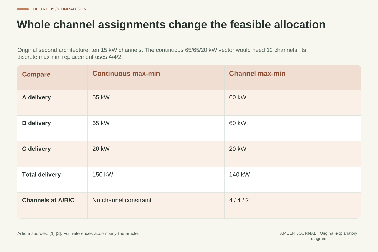
The earlier continuous allocation of 65, 65 and 20 is impossible under these new rules. A needs five channels to have capacity for 65, B also needs five, and C needs two for 20: twelve channels in total, when only ten exist. This does not mean delivery must occur in fifteen-kilowatt steps. Two channels assigned to C provide thirty of capacity while C can still draw only twenty. The indivisible item is the channel assignment, not every possible delivered power value.
Define integer assignments m_A,m_B,m_C≥0 with m_A+m_B+m_C≤10. Each assigned channel supplies up to 15 kW of capacity to exactly one port. Delivered power additionally obeys p_i≤15 kW×m_i and p_i≤u_i, and may vary continuously below those bounds. The manufacturer material motivates considering modular distribution, but neither this 15 kW architecture nor its routing rule is attributed to a real product. [1][2] We have changed the feasible set rather than merely rounded the earlier answer.
The continuous vector requires at least ceiling(65/15)=5 channels at each of A and B and ceiling(20/15)=2 at C. Their sum is 12, exceeding the available ten. Aggregate delivered power of 150 kW is therefore insufficient to establish feasibility in this architecture. Conversely, assigning two channels to C gives capacity 30 kW without requiring p_C=30 kW; its request still caps delivery at 20. Confusing assigned capacity with full output would incorrectly force a request violation and misrepresent the discrete constraint.
The allocation objective can change whether all capacity is used
Apply the same smallest-share-first objective to the channel system. C can never receive more than 20, and needs two channels to reach that request. Eight channels remain for A and B. Dividing them four each gives 60, 60 and 20 kilowatts. All ten channels are assigned, but delivery totals only 140. Ten kilowatts of capacity assigned to C are unused. That spare portion cannot move independently to another port under the model's whole-channel routing rule.
A different assignment uses six channels for A, three for B and one for C. It delivers 90, 45 and 15, using all 150. Total output is higher, but the smallest share falls from 20 to 15. This is why maximizing aggregate power and raising the smallest served shares are different objectives. Moving C's second channel elsewhere can release a whole channel, but it also lowers C's available capacity. The example compares declared mathematical choices; it does not prescribe a fairness policy for an actual charging site.
Lexicographically maximize the sorted delivered-power vector in the discrete architecture. The smallest share cannot exceed 20 kW because C is capped there. Achieving that value requires m_C≥2, leaving at most eight channels for A and B. Maximizing their smaller share then requires four channels each, producing p=(60,60,20) kW. Its sorted vector is (20,60,60), and its total is 140 kW. The corresponding capacities are (60,60,30) kW, so unused assigned capacity is 10 kW at C.
The assignment m=(6,3,1) instead delivers (90,45,15) kW and reaches the aggregate upper bound of 150 kW. It maximizes total throughput but has a smaller minimum share; it is one possible throughput maximizer, not a unique allocation. Exact enumeration of all 286 nonnegative integer assignments using at most ten channels confirms these results. The unused 10 kW under the max-min choice is not conversion loss or missing demand: it follows from whole-channel assignability combined with the chosen objective. Changing that objective or architecture changes the problem.
A complete time record is still needed to calculate charging energy
Return to the continuous model for a separate ten-minute record. For the first five minutes, delivery is 65, 65 and 20 kilowatts. For the next five, only C's request changes to ten, giving delivery of 70, 70 and 10. A receives 65 times five plus 70 times five kilowatt-minutes. Dividing that total by sixty gives 11.25 kilowatt-hours. B receives the same amount; C receives 2.5. Across all three, the delivered DC energy is 25 kilowatt-hours during this complete record.
The common output stayed at 150 kilowatts throughout those ten minutes, even though individual powers changed. Its total alone therefore cannot reveal each vehicle's energy without the allocation history. Nor does delivered DC energy automatically equal extra stored battery energy: the boundary here is the vehicle interface, and no internal loss or auxiliary account is supplied. The assigned request change also does not predict how long any vehicle needs to reach a target charge. That would require the remaining energy requirement and its later supported power history.
For an original two-interval trace, stipulate p=(65,65,20) kW on [0,5) min and p=(70,70,10) kW on [5,10) min. Integrating per port gives E_A=E_B=(65+70)×5/60=45/4 kWh and E_C=(20+10)×5/60=5/2 kWh. Their sum is 25 kWh, matching 150 kW×10/60 h. The proportional and discrete-channel alternatives are not mixed into this trace; it uses only the continuous progressive-filling rule with the declared changing request. These are output-energy totals for the three named ports.
A constant aggregate output does not imply constant individual powers or identify their integrals without allocation information. Likewise, these DC-interface energies are not necessarily stored-energy increments. Vehicle-side auxiliaries and internal losses would belong in an additional account, while time-to-target would require a target and subsequent request trajectory. The two intervals are invented, with ideal tracking and no switching delay; no communication response, converter transient or measured charging curve is represented. This keeps the exact integral useful without turning it into an unsupported session-performance prediction.
Read the budget, demands and policy together
A useful shared-charging description names the vehicle ports, the common power boundary, the available group budget and the limits of each requested output. It also identifies the allocation policy and any physical restrictions on moving capacity between outputs. The actual configuration matters in the ChargePoint architecture description, and the manufacturer charging explanation preserves the vehicle's role in requested power. [2][4] These facts are more informative than treating every connector label as an independent promise.
Our examples show the consequences. The same 150-kilowatt budget supports several continuous allocations, a capped equal quota can leave thirty unused, and satisfying all requests can leave capacity unused for a different reason. Whole channel assignments add another constraint: 65, 65 and 20 becomes infeasible even though its sum is 150. A complete record must then attach the chosen allocation to time before reporting energy. Keeping those inputs visible lets a reader distinguish a rating, a feasible limit, a policy decision and an actual session observation.
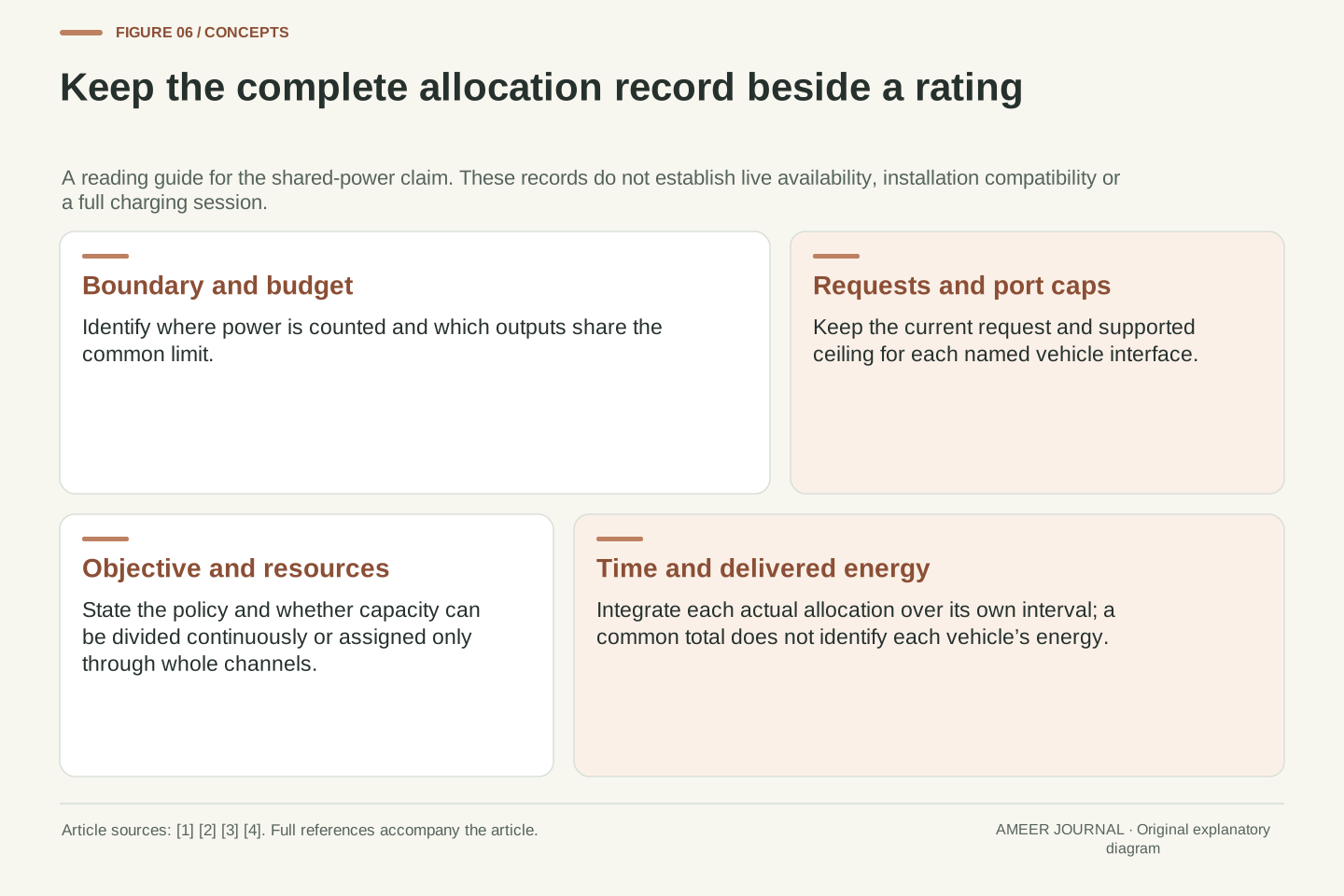
Retain six pieces of information: the common measurement boundary, aggregate budget, per-port/request caps, allocation objective, assignable resources and time history. Configuration dependence and varying vehicle requests are supported by the actual manufacturer documents, while AFDC distinguishes the named physical interfaces. [2][3][4] None of those facts alone identifies an implementation's precise allocation rule or proves that a particular advertised operating point is simultaneously feasible across all ports.
The original continuous model separates feasibility from selection through progressive, proportional and priority rules. The discrete model then adds integer channel constraints and shows why maximizing the smallest shares can differ from maximizing total power. Finally, the two-interval account distinguishes power allocation from delivered energy. These conclusions concern the stipulated models; they establish no live availability, queue delay, tariff, battery gain or hardware compatibility. They provide a precise way to ask which missing constraint or policy must be known before turning a shared cabinet's rating into an expectation for one connected vehicle.
Sources & further reading
Explore the references behind this guide. External pages may change after our review.
- The Benefits of Choosing Dynamic Power for Public EV Charging Sites - KempowerKempower · Accessed 7 Nov 2026
- IntroductionChargePoint · Accessed 7 Nov 2026
- Alternative Fuels Data Center: Electric Vehicle Charging StationsU.S. Department of Energy — Alternative Fuels Data Center · Accessed 7 Nov 2026
- How DC fast charging really works and an intro to charging curves | ChargePointChargePoint · Accessed 7 Nov 2026
Article updated 7 Nov 2026.
Found something we should revisit?
Good explanations get better with thoughtful feedback.