What you’ll take away
- A tyre can dissipate energy through repeated deformation without obvious sliding.
- The rolling-resistance coefficient is a force-to-normal-load ratio, not a vehicle energy percentage.
- At fixed rolling force, higher speed requires more power but the same rolling work per distance.
- A component improvement changes the whole account in proportion to that component's share, if other terms stay fixed.
- Consumption, range, grip and wear need their own denominators, conditions and supporting evidence.
A tyre can lose energy without visibly sliding
A car travels steadily along a level road. Its tyres turn smoothly, and no rubber seems to be scraping across the surface. Why must the powertrain still supply energy to keep those tyres rolling? A loaded tyre continually changes shape where it meets the road. Rubber does not return every bit of the mechanical energy used to deform it. Much of that unrecovered energy becomes heat, creating rolling resistance even without obvious sliding [1][4]. The loss occurs as new parts of the tyre repeatedly enter and leave the contact region.
That mechanism explains why a rolling-resistance improvement is useful. It does not, by itself, tell us the percentage improvement in the entire car's energy consumption. We will follow one hypothetical set of tyres from a force ratio to work over a kilometre, then place that work inside a larger energy budget. All numerical cases are invented teaching examples, not tyre measurements or performance promises. The result is a way to interpret an efficiency claim: identify the quantity that changed, the conditions behind it and the total against which its saving is being compared.
Rolling without gross sliding does not imply zero mechanical dissipation in a pneumatic tyre. Each rotation loads and unloads material around the contact region. Viscoelastic deformation produces a loss between mechanical energy supplied during loading and recovered during unloading; much of that loss appears as heat [1][4]. A resisting force or moment can represent this dissipation in a vehicle model, although the physical mechanism is distributed through a deforming tyre rather than located at one imaginary sliding point.
This article follows that effective loss through three distinct quantities: the rolling-resistance coefficient, the mechanical work required over a distance, and the fractional change in a complete energy account. The original examples assume level travel and explicitly stated loads, coefficients and accounting boundaries. They contain no measured product data. The key question is why reducing a component's loss by a particular percentage does not establish the same percentage reduction in whole-vehicle consumption. Answering it requires both the tyre mechanism and the denominator of the claimed improvement; a coefficient alone supplies neither a complete vehicle model nor a range prediction.
The shape can recover while some energy does not
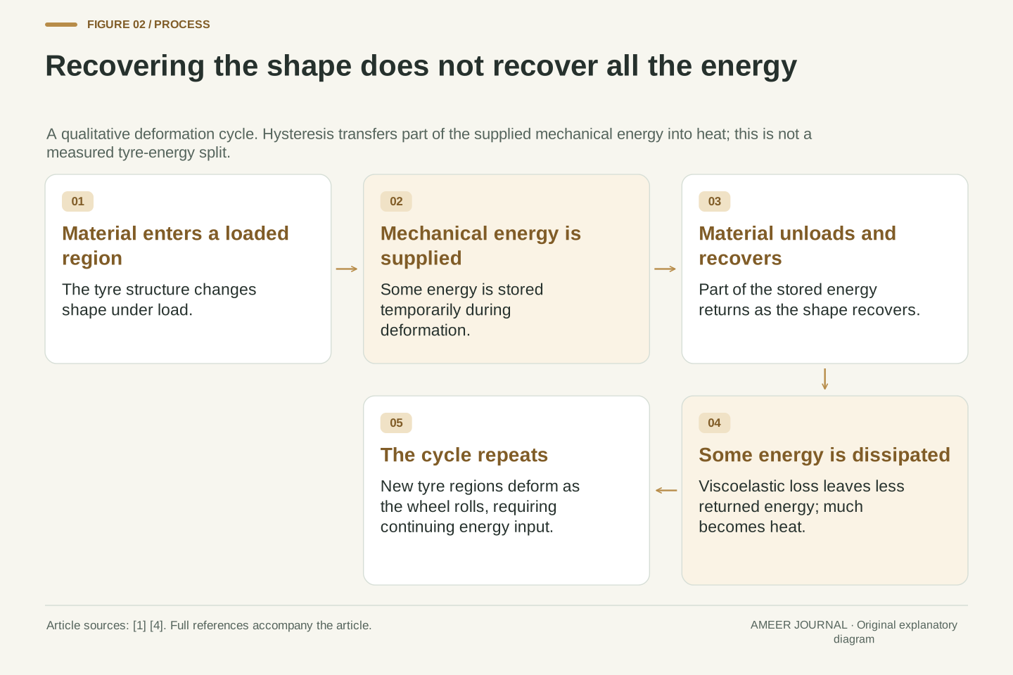
Imagine following one small region of rubber around a loaded wheel. As it approaches the road, the surrounding tyre structure bends and changes shape. After passing through the contact region, it recovers. An ideal perfectly elastic material would return all the energy temporarily stored during that change. Real tyre rubber combines elastic behaviour with time-dependent resistance to deformation. Some energy returns and some is dissipated. This repeating loss is called hysteresis [1]. Recovery of the visible shape therefore does not prove full recovery of the energy.
For a miniature energy account, suppose an imaginary deformation cycle receives 10 units of mechanical energy and returns 8. The missing 2 units have been transferred elsewhere, principally into heat in this simplified picture. That is a 20% loss within this invented cycle, not a 20% loss of the car's energy. Different tyre regions undergo different deformations, and the whole tyre combines those contributions. Material formulation, structure and geometry affect that response [1][2]. The example explains the mechanism without pretending that one small piece of rubber describes an actual tyre's measured efficiency.
Hysteresis describes the difference between work supplied during loading and recovered during unloading over a deformation cycle. In a force-displacement representation, the loop area corresponds to the mechanical energy dissipated per cycle. A purely elastic idealization has no such net loss when it returns to its original state; viscoelastic rubber need not recover the complete input work even when its macroscopic shape recovers [1]. The European Commission's explanation likewise identifies deformation-related hysteresis as a major rolling-loss mechanism [4].
For an original normalized cycle, W_in=10 units and W_return=8 units give W_loss=2 units. The cycle loss fraction is 2/10=0.20. Neither that fraction nor the drawn cycle can be substituted directly for a vehicle efficiency. The actual tyre integrates spatially varying deformation, material response and repeated cycles, while construction and compound choices influence those contributions [1][2]. A force-level representation is useful precisely because it summarizes the resulting loss under specified conditions. It must not be confused with the coefficient of sliding friction or treated as evidence that the contact patch is uniformly slipping.
The coefficient compares a resisting force with a normal load
The rolling-resistance coefficient compares the force needed to overcome rolling loss with the load pressing the tyre against the road. The load is measured perpendicular to the surface, which is why engineers call it the normal load [1][2]. If a hypothetical tyre carries 4,000 newtons and its rolling resistance is 40 newtons, the coefficient is 40÷4,000=0.010. The same ratio can be written as 10 newtons of resistance per kilonewton of load. It is not a statement that the tyre consumes 1% of the car's fuel or electricity.
Load matters alongside the coefficient. Another invented tyre with a smaller coefficient of 0.008, but a 6,000-newton load, has 48 newtons of rolling resistance. Its coefficient is lower, yet its force is higher than the first tyre's 40 newtons. For our main car example, stipulate a total tyre load of 16,000 newtons and the same coefficient, 0.010, at all four wheels. The total rolling resistance is then 160 newtons. There is no need to multiply that result by four again: the stated load already includes the whole set of tyres.
Define C_rr=F_rr/N, where N is the normal load and F_rr is the effective resistance magnitude under the stated conditions. Both numerator and denominator are forces, so C_rr is dimensionless [1][2]. A value of 0.010 is equivalent to 10 N/kN because 1 kN=1,000 N. Confusing N/kN with N/N introduces a factor of one thousand. The ratio normalizes a force; it is not an energy-efficiency percentage.
The hypothetical cases C_A=0.010, N_A=4,000 N and C_B=0.008, N_B=6,000 N give F_A=40 N and F_B=48 N. Coefficient ranking therefore need not rank unnormalized force. For multiple tyres, F_total=Σ(C_i N_i). If every C_i equals 0.010 and ΣN_i=16,000 N, then F_total=160 N. With unequal coefficients, the effective set coefficient is Σ(C_i N_i)/ΣN_i, a load-weighted average. An unweighted mean is justified only when the loads are equal or another special condition makes it equivalent. Load and coefficient must remain paired throughout the calculation.
A force becomes energy over distance and power over time
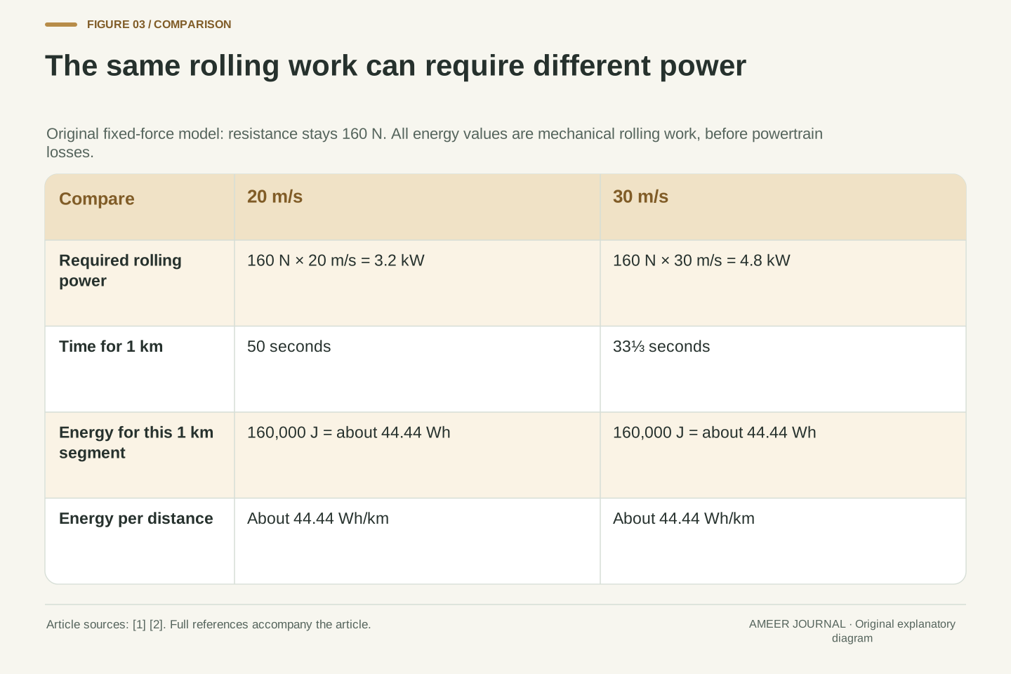
Apply the main example's steady 160-newton resistance over 1 kilometre. The mechanical work needed to overcome it is 160×1,000=160,000 joules. Dividing by 3,600 converts that energy to about 44.44 watt-hours. For this one-kilometre segment, the corresponding energy per distance is 44.44 Wh/km. The distinction matters: 44.44 Wh is the energy for the segment, while 44.44 Wh/km is the rate of energy use with distance. This account covers rolling resistance at the wheels, before any powertrain or charging losses.
Now hold both the load and coefficient fixed while changing speed. At 20 metres per second, the power needed is 160×20=3,200 watts. At 30 metres per second it is 4,800 watts. The faster trip needs more power, but each kilometre takes less time, leaving the same rolling work per kilometre in this model. That result comes from the fixed-force assumption; real tyre resistance can change with operating conditions, including speed and temperature [1]. It also says nothing about the car's other energy demands, which can change substantially when speed changes.
For constant effective resistance parallel and opposite to motion, the required positive work over path length s is W_rr=F_rr s. Thus 160 N over 1,000 m requires 160,000 J=44.444… Wh; normalized over that segment, the consumption is 44.444… Wh/km. For varying conditions the general account is W_rr=∫F_rr(s)ds. The resisting force itself does negative work on vehicle motion, while the equal sustaining contribution supplies positive work. Using the magnitude avoids reversing those two sign conventions.
At speed v, the sustaining power is P_rr=F_rr v. Holding F_rr=160 N yields 3.2 kW at 20 m/s and 4.8 kW at 30 m/s. Traversal times for 1 km are 50 s and 33⅓ s, respectively; P times duration gives 160 kJ in either case. Constant Wh/km follows from constant force, not from a universal property of tyres. The source review describes operating-state and speed-related influences on rolling resistance [1]. Changing coefficient, load or path conditions requires integrating the appropriate force rather than retaining this example's constant value.
Twenty percent less rolling loss is a smaller whole-budget change
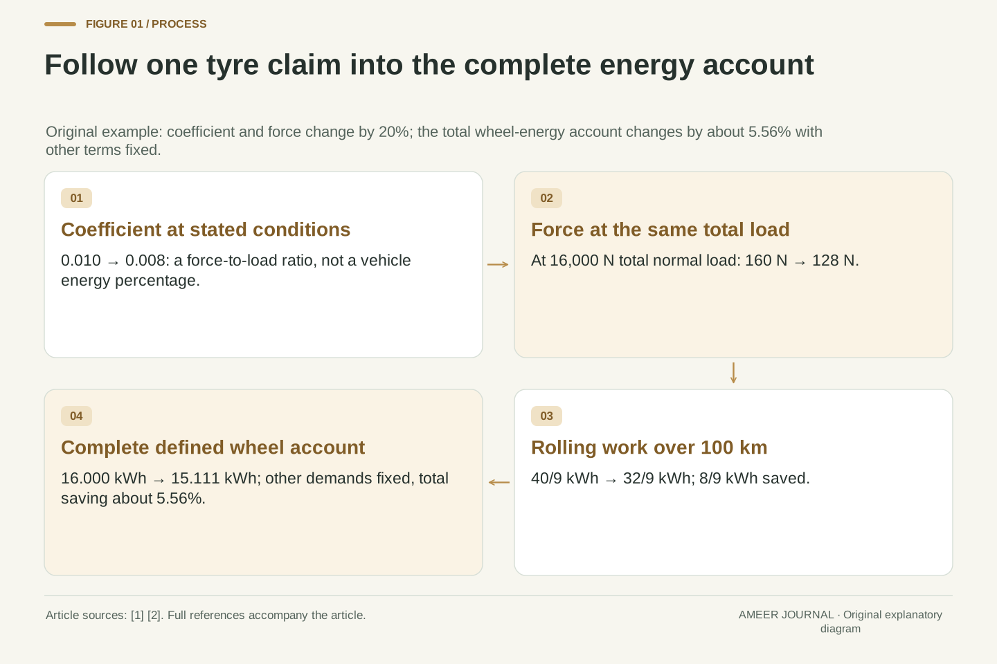
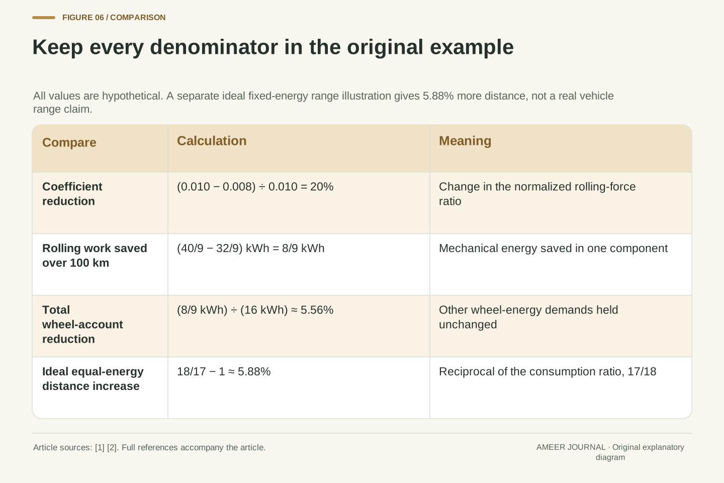
Keep the same 16,000-newton load, but change the hypothetical coefficient from 0.010 to 0.008. Rolling resistance falls from 160 to 128 newtons, a reduction of 20%. Over 100 kilometres, the rolling work falls from about 4.444 to 3.556 kilowatt-hours. The saving is about 0.889 kWh. These are mechanical energy amounts for the tyres' rolling loss, calculated from the stated force and distance. They do not yet describe energy taken from a battery or fuel tank.
Suppose a separately defined wheel-level account totals 16 kWh over that same distance. Of that total, 4.444 kWh is the rolling term; the remaining 11.556 kWh covers the other unchanged wheel-energy demands. Replacing only the rolling term gives 15.111 kWh. The total reduction is 0.889÷16, or about 5.56%. The 20% improvement is real within the example, but it acts on one part of the account. Vehicle-technology reports explain that the whole-vehicle benefit depends on the share of energy associated with rolling resistance and on the rest of the vehicle's losses [2].
With N_total=16,000 N, reducing C_rr from 0.010 to 0.008 reduces F_rr from 160 N to 128 N. The relative change is 0.002/0.010=20%. Over s=100,000 m, baseline and revised rolling work are 16.0 MJ and 12.8 MJ, or 40/9 kWh and 32/9 kWh. The saving is 8/9 kWh. This is an original mechanical-work calculation, independent of a chosen engine, motor or battery efficiency.
Define the complete baseline wheel account as E_total=16 kWh, including E_rr=40/9 kWh and E_other=104/9 kWh. Holding E_other fixed gives E_new=136/9 kWh≈15.111 kWh. The fractional total saving is (8/9)/16=1/18≈5.56%. More generally, reducing one loss by fraction r reduces the defined total by r×(E_rr/E_total), when the other terms and accounting boundary remain unchanged. This is the denominator effect behind the gap between component improvement and total improvement. The National Academies' discussion supports the need to retain vehicle energy shares and conversion losses [2]; its historical fleet percentages are not inputs to this example.
A controlled coefficient is a comparison under controlled conditions
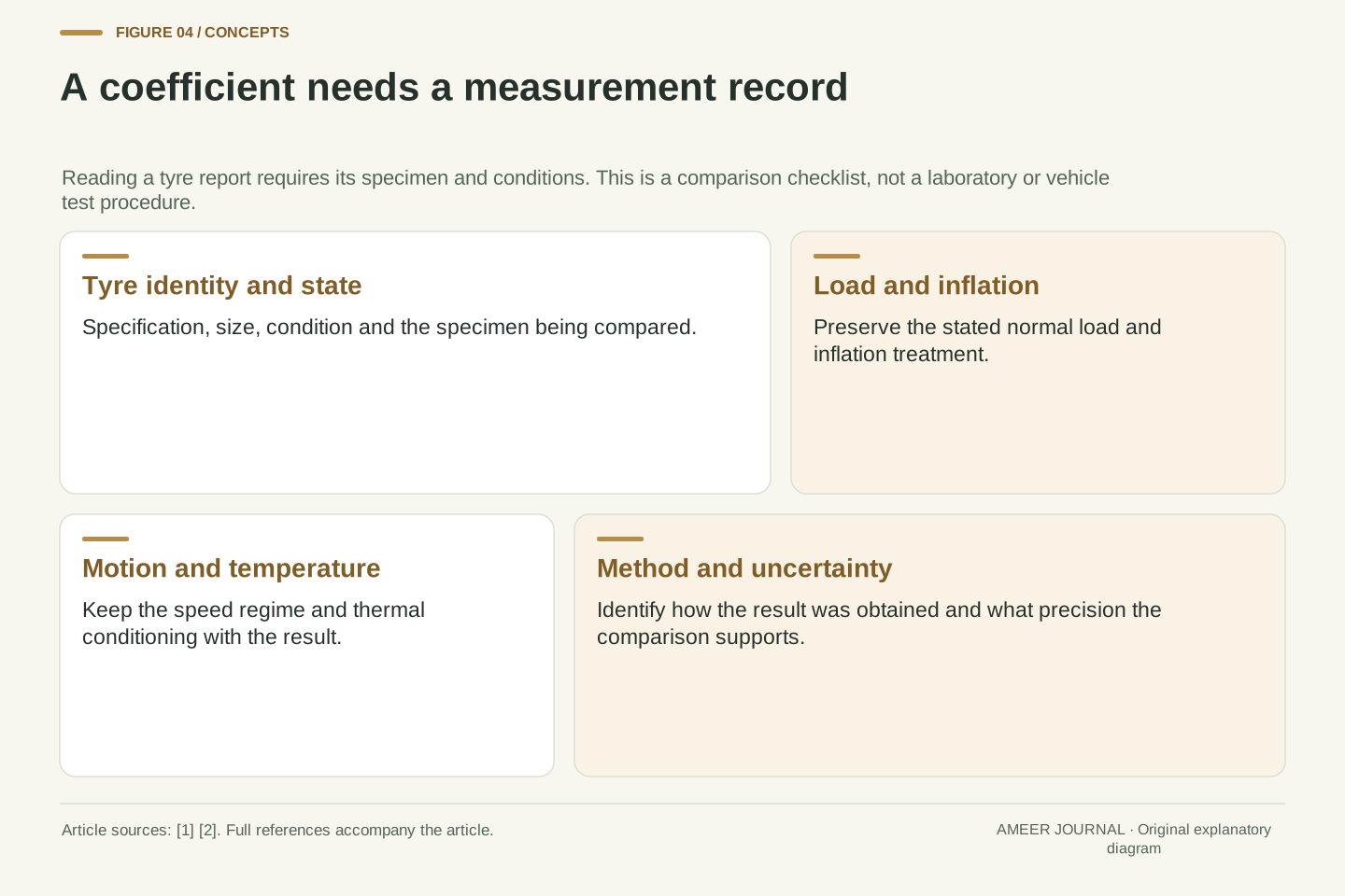
A tyre laboratory tries to isolate the property being compared. Load, inflation, temperature and the measurement procedure need suitable control; otherwise a different result may reflect a different condition rather than a better tyre. The Transportation Research Board's report explains why controlled rolling-resistance procedures improve repeatability and why laboratory results still differ from varied road experience [1]. A useful report therefore attaches conditions to the coefficient instead of presenting it as a timeless number belonging to the tyre in every situation.
Imagine two reports that both say 8 N/kN. One describes a stated new tyre under a controlled procedure; the other gives no size, condition or method. Their printed ratios match, but the second report does not establish that the underlying comparison matches. Conversely, two reported values may differ partly because the tyres or conditions differ. The questions to keep are concrete: what exact tyre was assessed, under what load and inflation conditions, with which method, and with what stated measurement uncertainty? These questions identify missing evidence without assuming that either result is dishonest or that a laboratory test predicts every journey.
A rolling-resistance measurement is conditional on the test specimen and procedure. Controlled methods support repeatability and instrumentation accuracy by specifying operating conditions, yet the source report explicitly distinguishes laboratory comparability from the diversity of field conditions [1]. Its 2006 discussion is used here for that enduring measurement principle, not as a claim about the latest edition or legal status of a particular test standard.
An interpretable record identifies tyre specification and state, imposed load, inflation treatment, speed regime, thermal conditioning, measurement method and uncertainty where available. Equality of two reported coefficients is not enough to establish equality of the measurands if those conditions differ. Likewise, a numerical difference does not establish a material advantage without the procedure's uncertainty and comparability. In our example, C_rr=0.010 and 0.008 are stipulated model inputs. They are not inferred from a label class, a current catalogue or a vehicle's displayed consumption. Preserving that distinction keeps a clean worked calculation from being mistaken for a product comparison.
The same tyre can experience a different loss on another journey
A tyre's design is only one part of the rolling-loss story. Changing load or inflation changes how it deforms. Temperature affects the material response, and a rougher or more deformable road changes the interaction between tyre and surface [1]. A vehicle on another route or carrying another load is therefore not automatically repeating the same rolling-resistance experiment. The simple coefficient model remains useful, but its inputs must represent the situation being discussed.
Consider a small mathematical check. Keep the coefficient at 0.010 while increasing our car's total normal load from 16,000 to 18,000 newtons. Resistance rises from 160 to 180 newtons, or 12.5%. That follows under the declared constant-coefficient assumption. It does not prove that every real tyre responds by precisely that percentage, because the coefficient itself can vary with conditions. Nor does the model justify changing inflation to chase a calculated minimum. NHTSA directs owners to the vehicle's tyre information label or owner's manual for the specified pressure [3]. The operating recommendation and an energy-model parameter serve different purposes.
The approximation F_rr=C_rr N is useful across a declared operating range, but C_rr can itself depend on load, inflation, temperature, speed, construction and road interaction. The source review describes near-proportional force-versus-load behaviour under normal conditions while also identifying important operating variables and surface influences [1]. The coefficient is therefore not a universal constitutive constant independent of state.
For a sensitivity calculation with C_rr held at 0.010, increasing N_total from 16 kN to 18 kN gives 160 N to 180 N: a 12.5% increase. If the coefficient changes as well, the ratio is F_new/F_old=(C_new/C_old)×(N_new/N_old). Keeping both factors makes the assumption visible. Road roughness can also affect energy pathways outside a narrow isolated-tyre laboratory description, so a whole-vehicle road result requires an explicit boundary. These dependencies motivate proper model inputs; they are not instructions to optimize inflation independently of vehicle requirements. NHTSA identifies the vehicle label or manual as the pressure reference [3].
Energy saved and distance gained use different denominators
Our 5.56% reduction belongs to a specified mechanical energy account. To predict battery consumption, fuel use or electricity at a charger, we would also need the relevant conversion losses and other demands. A heater, for example, is not part of the defined wheel-work ledger. The National Academies describes different vehicle energy pathways and explains why rolling-loss changes do not translate into one universal consumption response [2]. Moving a result from one boundary to another needs additional information.
There is a second arithmetic trap even when the boundary is fixed. Imagine an ideal system with the same available 16 kWh in both cases and energy per distance exactly proportional to our wheel account. The baseline allows 100 kilometres; the revised 15.111 kWh per 100 kilometres allows about 105.88 kilometres. The energy-per-distance reduction was 5.56%, but the distance increase is 5.88%, because distance is divided by consumption. This separate hypothetical exercise is not a real range estimate. It shows why 'percent less energy per kilometre' and 'percent more kilometres' need not be numerically identical.
A change in mechanical wheel work cannot simply be relabelled as an equal fractional change in fuel, battery-terminal or wall energy. Conversion efficiencies, accessory loads and operating profiles affect the mapping, and the cited vehicle-energy discussion separates those pathways [2]. Even a constant efficiency would preserve a fractional improvement only for the terms to which it applies, with no additional unchanged energy demand entering the denominator.
For a separate ideal fixed-energy illustration, consumption changes from e_0=16 kWh/100 km to e_1=136/9 kWh/100 km. Their ratio is e_1/e_0=17/18, so the consumption reduction is 1/18≈5.56%. At equal available energy and otherwise identical conditions, distance is inversely proportional to e: D_1/D_0=18/17. Its increase is 1/17≈5.88%. With an invented 16 kWh allowance, the distances are 100 km and 1,800/17 km≈105.88 km. The different denominators explain the unequal percentages; neither number is a measured EV range benefit or an assertion that usable battery energy equals wheel work.
A rolling-loss score does not supply a grip or wear score
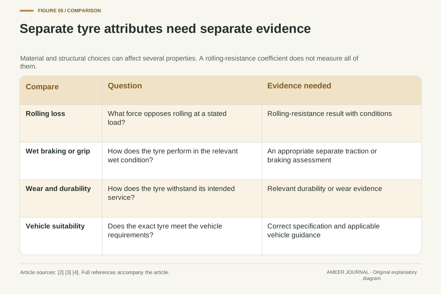
A tyre must do more than roll with low loss. It must support the vehicle and provide suitable braking, traction, handling and durability. NHTSA lists several performance attributes influenced by materials, construction and tread design [3]. The National Academies and European Commission also discuss the competing demands involved in tyre design [2][4]. A lower rolling-resistance coefficient therefore answers one performance question; it does not reveal a complete set of answers about the tyre.
This cuts both ways. A lower coefficient does not prove poor wet grip, and a high coefficient does not prove excellent grip. Those properties need their own relevant evidence. Similarly, less rubber deformation in one design cannot be turned into a recommendation to remove tread or change the specified fitment. A comparison should retain the tyre's exact specification and separately supported attributes. The practical value of understanding rolling resistance is that it lets you recognize a real efficiency measure while refusing to make unrelated conclusions from it. An energy benefit can be considered alongside safety and service requirements without pretending that one number replaces them.
Rolling resistance is one response within a multidimensional design problem. The source documents identify wet and dry traction, braking, handling, ride, durability and noise as distinct considerations, with material and structural choices influencing more than one response [2][3][4]. Interactions and trade-offs do not establish a universal one-to-one relationship between C_rr and any other performance metric. An individual design can change several variables at once.
Consequently, C_rr cannot serve as a surrogate measurement for wet braking distance, wear life or suitability for a particular vehicle. A comparison requires the correct tyre specification and independent evidence for the properties that matter to the intended use. This is also why the article does not translate historical tread-wear experiments into owner advice or infer current regulatory label classes from its invented coefficients. The model's 20% rolling-loss reduction is conditional on its inputs and load. It neither certifies a tyre nor assigns a penalty to an unmeasured property. Separating the questions makes the efficiency result more useful rather than less credible.
A consumption display cannot isolate the tyre by itself
Suppose a driver changes tyres and later sees a lower average consumption figure. The observation can be real without showing how much of the change came from rolling resistance. Route, speed, wind, traffic, payload, temperature and accessory use may also have changed. Laboratory controls exist partly because ordinary journeys combine many influences [1]. A single before-and-after display gives a total result; it does not separately measure each contribution inside that total.
The useful distinction is between observation and attribution. 'Consumption was lower on this journey' describes what was recorded. 'The tyres alone caused the entire difference' requires evidence that rules out the other explanations. Our calculation avoids that problem by stipulating unchanged other demands, which is why its 5.56% result follows cleanly. For a real report, look for comparable conditions, a stated method and repeated evidence with uncertainty. This is a way to read a claim, not an invitation to perform road tests, coast in traffic or change tyre settings. A good comparison makes its controls visible instead of hiding them behind a precise percentage.
Whole-vehicle consumption is an aggregate observable. Estimating the causal contribution of a tyre change requires controlling or modelling competing changes in route, aerodynamic demand, vehicle loading, thermal state and accessories. The source report explicitly warns that varied road surfaces, inflation, alignment and other operating conditions affect field rolling resistance and its agreement with laboratory values [1]. A raw consumption difference does not uniquely identify ΔC_rr.
For the worked budget, attribution is possible because E_other is fixed by construction. In observational data it is an assumption to evaluate, not a fact supplied by the display. Even with matched reported averages, differing speed distributions or thermal histories can change the underlying demands. A defensible comparison needs an identified protocol, compatible tyre specifications, sufficient repeated evidence and appropriate uncertainty treatment. The article proposes no on-road experiment. Its purpose is to distinguish a measured aggregate change from a modelled component contribution, and to explain why a precise result without those controls can be less informative than a carefully bounded range.
Read the coefficient, the work and the total as separate quantities
Return to the headline claim: a tyre set has 20% less rolling resistance. First ask whether that means a lower coefficient under comparable conditions or a lower force at the same load. Then ask how the claim becomes energy over a specified distance. Finally, ask which complete energy account is being used. Those three steps prevent a component result from quietly becoming a whole-car promise.
In our example, 0.010 becoming 0.008 at a total 16,000-newton load reduces the force from 160 to 128 newtons. Over 100 kilometres it saves about 0.889 kWh of rolling work. Inside the stipulated 16 kWh wheel account, that is about 5.56%, with every other term unchanged. The mechanism is repeated deformation; the measure is force relative to load; the benefit depends on the larger denominator. Keep those pieces together, alongside the tyre's other independently supported properties and the vehicle's specified operating requirements [1][2][3]. You can then recognize both the real value of lower rolling loss and the extra evidence needed to predict a particular car's consumption.
A complete interpretation retains the sequence C_rr→F_rr→W_rr→ΔE_total/E_total. Each step introduces information: normal load, distance or operating trajectory, and the remainder of the energy account. The original fixed-load case gives 0.010→0.008, 160→128 N and 40/9→32/9 kWh over 100 km. At E_total=16 kWh with other terms fixed, the total fractional saving is 1/18. The coefficient change alone does not encode that final denominator.
For a real claim, preserve specimen, method, conditions, physical boundary and uncertainty, then assess other tyre attributes independently [1][2][3]. If a range statement is added, also identify usable energy and the reciprocal consumption relation. This reading discipline does not require an elaborate vehicle simulation merely to understand the claim. It identifies exactly where further evidence becomes necessary. Rolling resistance is a physically meaningful energy loss in a deforming tyre; its coefficient is a useful normalized measure. The mistake is to let that one measure silently stand in for every energy pathway or every performance requirement of the vehicle.
Sources & further reading
Explore the references behind this guide. External pages may change after our review.
- Read "Tires and Passenger Vehicle Fuel Economy: Informing Consumers, Improving Performance -- Special Report 286" at NAP.eduTransportation Research Board / National Academies · Accessed 6 Nov 2026
- Read "Assessment of Technologies for Improving Light-Duty Vehicle Fuel Economy—2025-2035" at NAP.eduNational Academies of Sciences, Engineering, and Medicine · Accessed 6 Nov 2026
- Tire Safety Ratings and Awareness | TireWise | NHTSAU.S. National Highway Traffic Safety Administration · Accessed 6 Nov 2026
- Tyres properties: an introduction - Energy Efficient ProductsEuropean Commission · Accessed 6 Nov 2026
Article updated 6 Nov 2026.
Found something we should revisit?
Good explanations get better with thoughtful feedback.