What you’ll take away
- A following setting, measured time headway and constant-speed closing time are different quantities.
- The same gap and follower speed can accompany closing, unchanged or increasing separation.
- A time coefficient in a distance policy need not equal the actual gap divided by speed.
- Changing targets, acceleration and support availability can invalidate a snapshot-based prediction.
- ACC remains bounded driver assistance; these paper calculations are not safe-gap settings or road tests.
A following interval is not a countdown to contact
An adaptive-cruise display can show a chosen following interval while the distance to the vehicle ahead is changing. That interval is not a promise that a collision is a fixed number of seconds away. Adaptive cruise control, or ACC, adjusts speed in relation to a vehicle detected ahead; Transport Canada describes both distance and relative speed as inputs to this task [1]. To understand the display, separate how much space exists, how quickly that space is changing and what the system is trying to maintain.
This article uses original paper calculations, not a road test or a vehicle-control simulation. Every numerical speed, gap, delay and braking rate is invented. None is a recommended setting, a legal following interval or a measured driver or system response. We first compare two different time quantities, then show why equal speeds and a familiar gap do not establish a stopping guarantee. Specific Polestar and Volvo manual pages provide examples of documented behavior, with their vehicle and market boundaries retained. The calculations explain the questions to ask; the exact vehicle guidance and actual conditions govern driving.
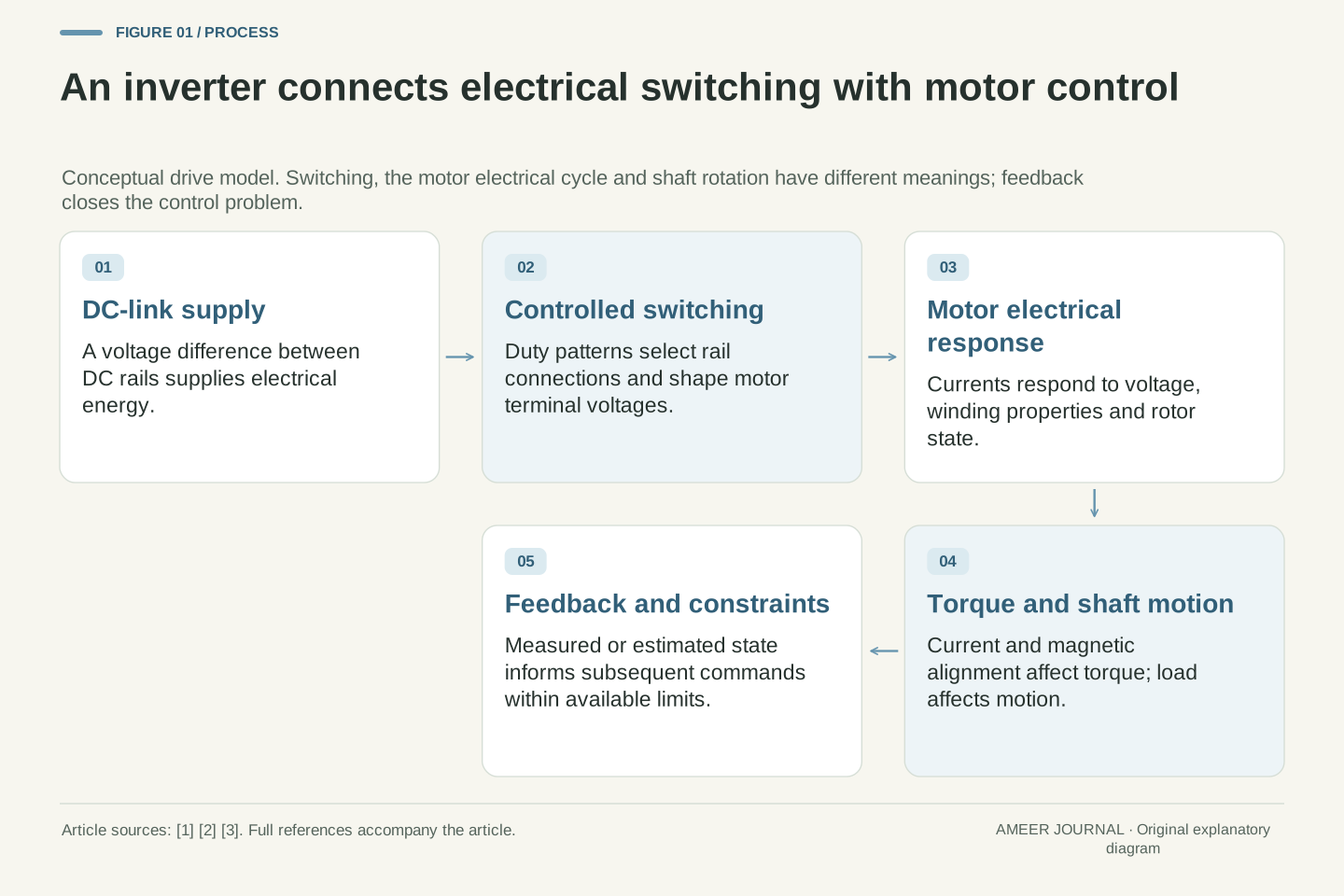
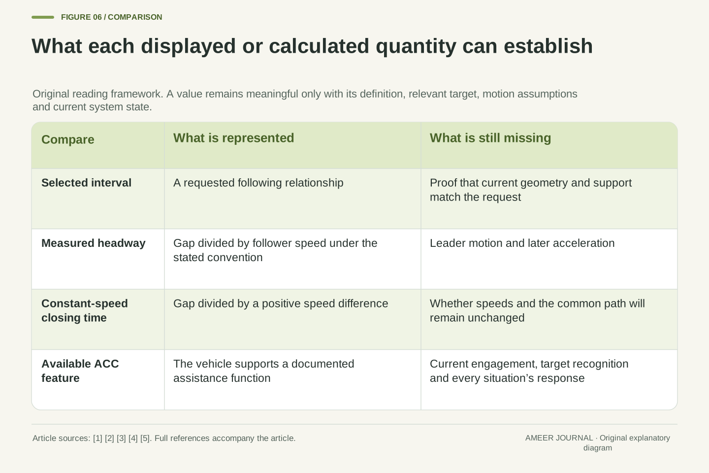
A selected ACC following interval, a measured time headway and a constant-velocity time to contact are different quantities. The function uses lead-vehicle information to regulate longitudinal motion; Transport Canada's account explicitly includes range and relative speed [1]. A displayed interval is therefore a control-related setting or state indication, not by itself a complete prediction of the future separation trajectory.
The original models below are one-dimensional and use bumper-to-bumper gap d, follower speed vf and lead speed vl along a common straight path. Positive gap means physical separation. All numerical inputs are hypothetical, with no real vehicle, driver, controller implementation or road test represented. The mathematical examples are not prescriptions for safe or lawful headway. They isolate missing information: relative velocity, changing acceleration, target identity and active support state. Specific manufacturer pages illustrate why those distinctions matter without supplying a universal operating algorithm. A control target should never be substituted for evidence that every condition needed for that target is currently satisfied.
Set speed and following behavior answer different questions
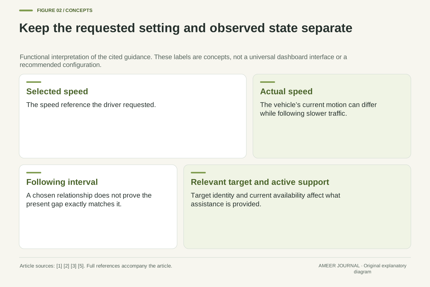
Conventional speed control aims at a selected speed. ACC adds a following task: when a relevant vehicle ahead is slower, the system can reduce the follower's speed to maintain separation. When there is no such vehicle to follow, it can return toward the selected speed [1][2]. The selected number and the speed actually being driven can therefore differ without either display being broken.
Imagine a selected speed of 25 metres per second while the followed vehicle travels at 20 metres per second. Matching the slower vehicle can be part of ordinary following behavior. The 25 figure is a reference for the speed-control task, not proof that the car is currently travelling at 25. It is also not an independent promise of a hard speed ceiling under every condition. A useful reading keeps the selected speed, actual speed, current target and following setting separate. Otherwise, a change caused by traffic can be mistaken for a change in the driver's selected reference.
ACC combines a speed reference with a following constraint or objective. NHTSA defines the function by automatic speed adjustment to maintain a preset distance, while Transport Canada describes the return toward selected cruising speed when no vehicle is being followed [1][2]. This is a functional description, not a claim that every implementation uses the same switching logic or control architecture.
In the invented case v_set=25 m/s and vl=20 m/s, a follower travelling at 20 m/s may be responding to the lead vehicle rather than tracking the unconstrained speed reference. Neither the reference nor a selected interval establishes the instantaneous actuator command. A real controller's response also depends on its estimates, limits and operating state. Treating the set speed as a guaranteed hard ceiling would add a property not established by this account. The important distinction is between a requested reference, an observed state and the assistance currently being applied. They can legitimately have different values and meanings.
The same time headway corresponds to more metres at higher speed
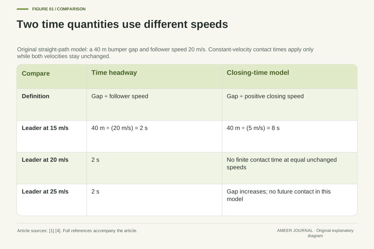
Define an observed time headway by dividing the current gap by the follower's current speed. With a 40-metre gap and a speed of 20 metres per second, the result is two seconds. It describes how long the follower would take to cover that distance at that unchanged speed. It does not account for where the other vehicle will move during those two seconds. This is a definition applied to our drawing, not a claim about a particular car's displayed calculation.
Under a pure two-second distance rule, speeds of 15, 20 and 30 metres per second correspond to gaps of 30, 40 and 60 metres. The chosen time is unchanged while the physical distance grows. The 2025 Australian Polestar 2 manual similarly explains that a given time interval corresponds to a longer distance at higher speed [3]. Its own controls and display mapping are vehicle-specific. Do not read a bar as a fixed number of metres or transfer a bar-to-time meaning from one manufacturer's display to another.
For vf>0, define measured net time headway H=d/vf using the chosen bumper-gap convention. At d=40 m and vf=20 m/s, H=2 s. This is a kinematic ratio, not a future interception calculation. The leader's velocity does not appear in its denominator. Other transport definitions can include different reference points; the convention must stay explicit when comparing quantities.
A pure constant-headway target d*=T vf with T=2 s gives 30, 40 and 60 m at vf=15, 20 and 30 m/s respectively. Polestar's specified 2025 Australian manual supports the qualitative speed-to-distance relationship and also notes that maintained intervals can vary in some circumstances [3]. We do not identify this simple equation as its production controller. At vf=0, the measured ratio d/vf is undefined, even when a finite standstill gap exists. That alone shows why a time-based description needs additional interpretation around stops rather than blind numerical division.
Closing time uses the speed difference between the vehicles
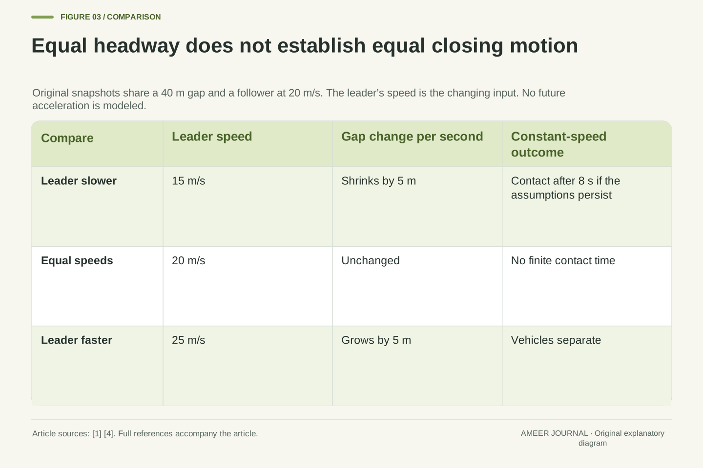
Keep the follower at 20 metres per second and the gap at 40 metres. If the leader is also moving at 20, the gap stays unchanged in the constant-speed drawing. There is no finite contact time under that assumption. If the leader instead travels at 15, the follower gains five metres each second. Dividing 40 by five gives eight seconds to contact if both velocities and their common path remain unchanged. Both cases begin with the same two-second headway.
A third leader moving at 25 metres per second pulls away from the same follower, so the gap grows. Writing a negative collision countdown would be misleading; the constant-speed model predicts no future closing contact. These examples use basic position-versus-time relationships [4]. They also expose the limit of the eight-second result: it stops applying when either vehicle accelerates, brakes or changes path. An instant with no closing speed is a description of present relative motion, not evidence that the situation cannot become hazardous.
A separate invented case starts with both speeds at 20 metres per second and the same 40-metre gap. Now let the leader lose two metres per second of speed each second while the follower keeps its speed. After three seconds the gap is 31 metres and the closing speed is six metres per second. Holding those current speeds would suggest about 5.17 seconds remaining. Continuing the stated slowing pattern instead brings the model gap to zero about 3.32 seconds later. The different answers come from different future-motion assumptions, not from an arithmetic error.
Let closing speed c=vf−vl. With fixed velocities and a common path, d(t)=d0−ct. For d0>0 and c>0, the first zero is TTC=d0/c. At d0=40 m, vf=20 m/s and vl=15 m/s, c=5 m/s and TTC=8 s, while measured headway remains H=2 s. The linear propagation follows the constant-velocity case of the kinematic relationships [4].
For vl=20 m/s, c=0 and the positive gap does not reach zero under that model; TTC has no finite value. For vl=25 m/s, c<0 and the gap increases, so a negative quotient is not a future collision time. The formula also requires continued common-path relevance. It does not predict a lane change or a new target. With changing acceleration, one must propagate the relative motion using those additional inputs. Neither a large TTC nor a currently undefined finite TTC certifies that later braking demand will remain manageable.
For another original constant-acceleration case, initially set vf=vl=20 m/s,d0=40 m,af=0 and al=−2 m/s². While these conditions persist, d(t)=40 m−(1 m/s²)t². At t=3 s, d=31 m and c=6 m/s, giving an instantaneous constant-velocity TTC of 31/6 s≈5.167 s. Yet continuing the acceleration model produces zero gap at t=√40 s≈6.325 s from the start, only 3.325 s after that snapshot. Both vehicles remain moving forward until contact in this ideal calculation. The mismatch shows that an updated quotient still assumes unchanged future velocities; it does not incorporate a known continuing acceleration. No physical trajectory beyond contact is represented.
A time coefficient and a measured interval need not be identical
A simple invented distance policy adds a fixed five-metre allowance to one and a half seconds of travel. At 20 metres per second, that means 5 plus 30, or 35 metres. Dividing the resulting gap by speed gives 1.75 seconds, even though the policy's time coefficient is 1.5 seconds. The extra fixed distance explains the difference. This is a teaching model, not a decoded Polestar, Volvo or other vehicle setting.
At 10 metres per second the same policy gives 20 metres, equivalent to two seconds by our measured ratio. At 30 it gives 50 metres, or about 1.67 seconds. At rest it still asks for five metres, while distance divided by zero has no time value. A setting, a policy coefficient and a measured gap can therefore differ for understandable reasons. The Polestar manual's warning that maintained intervals can vary [3] is a further reason to read the actual documentation instead of assuming one fixed arithmetic rule describes every situation.
Matching the requested distance at one instant also need not mean a settled following condition. In the invented policy, if the follower begins gaining speed, the requested gap grows too. A calculation must follow that changing target as well as the actual space between the vehicles. A correct snapshot can therefore be the start of a change rather than the end of an adjustment.
Consider the explicitly invented policy d*=d_s+T vf with d_s=5 m and T=1.5 s. At vf=0,10,20,30 m/s, target distances are 5,20,35,50 m. For positive speeds, the associated measured ratio is d*/vf=T+d_s/vf, yielding 2,1.75 and 5/3 s for the three nonzero cases. The finite offset changes the ratio without changing T.
This policy illustrates definitions rather than identifying a real ACC law. Its distance error e=d−d* has rate e_dot=vl−vf−T af when d_s and T are constant and af is follower acceleration. Even in this simplified model, matching a target distance is not the same as matching relative velocity or holding a fixed target forever. A real controller adds estimation, actuation and constraints that are not specified here. The documented possibility of variable maintained intervals [3] should not be mistaken for proof of this particular equation or any inferred tuning parameter.
For example, at vf=vl=20 m/s and d=d*=35 m, instantaneous relative velocity is zero. If the follower acceleration at that instant is 1 m/s², the target-distance rate is 1.5 m/s and e_dot=−1.5 m/s. Zero distance error at that instant does not establish equilibrium: the reference itself is moving in state space. This is a derivative of the invented policy, not a claimed real controller command.
A cut-in changes the target as well as the gap
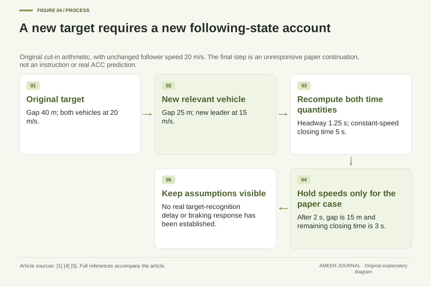
Begin with both vehicles travelling at 20 metres per second and separated by 40 metres. Now replace the followed vehicle in the drawing with a newly relevant vehicle 25 metres ahead, travelling at 15 metres per second. The new measured headway is 1.25 seconds and the constant-speed closing time is five seconds. The old target's unchanged gap history no longer describes the new target. No mathematical inconsistency is required for the displayed situation to change quickly.
If those new velocities were held for another two seconds without any response, the gap would shrink by ten metres to 15. The remaining constant-speed closing time would then be three seconds. This is a paper continuation, not an instruction to wait or a prediction of ACC behavior. Transport Canada explicitly identifies slower cut-ins and sharp lead braking as situations in which the driver may need to brake [1]. A previously comfortable following pattern cannot substitute for assessing the vehicle that is now relevant.
Target identity is part of the state being interpreted. The original pair has d=40 m,vf=vl=20 m/s. A new same-path target at d=25 m,vl=15 m/s changes the observed state discontinuously even though vf has not changed. Now H=(25 m)/(20 m/s)=1.25 s and the constant-velocity TTC is (25 m)/(5 m/s)=5 s. A historical estimate attached to the old target cannot simply be carried over.
Under the deliberately unresponsive constant-speed continuation, d(2 s)=25 m−(5 m/s)(2 s)=15 m; H becomes 0.75 s and TTC becomes 3 s. This propagates the stated trajectories only; it supplies no detection latency or braking response for a real vehicle. The primary guidance identifies cut-in and sharp-braking limitations [1], while Volvo's page says tracking depends on accurate detection and identification [5]. Separating target selection from gap arithmetic explains why a correct distance formula is insufficient to establish that the system has selected and will appropriately handle the relevant object.
Equal speeds can become an inadequate stopping arrangement
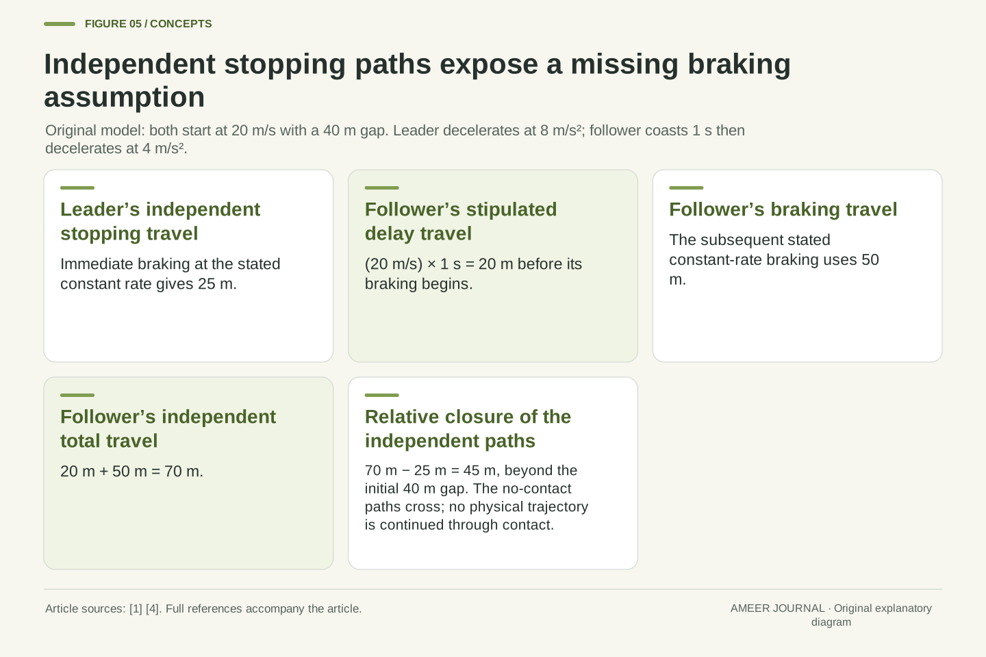
Return to the initial 40-metre gap with both vehicles at 20 metres per second. Give the leader an immediate constant slowing rate of eight metres per second per second. In our invented account, it takes 2.5 seconds and 25 metres to stop. Let the follower keep its speed for one second, then slow at four metres per second per second until stopped. Its first second uses 20 metres, and its later braking uses another 50 metres, for 70 metres in total.
The follower's independent stopping path is 45 metres longer than the leader's, while their initial gap was only 40 metres. Those independently continued paths would cross before both stopping plans finish. The initial two-second headway and zero closing speed did not prevent this mathematical counterexample. The rates and delay are assumptions, not actual braking strengths or a normal response time. The calculation uses constant-acceleration equations [4] to demonstrate missing information, and it establishes no alternative universally safe gap.
For a separate piecewise model, take d0=40 m and vf0=vl0=20 m/s. The leader decelerates at magnitude bl=8 m/s² immediately, so its stopping time is 2.5 s and displacement vl0²/(2bl)=25 m. The follower has a stipulated zero-acceleration delay τ=1 s, followed by constant deceleration magnitude bf=4 m/s². Its displacement is vf0τ+vf0²/(2bf)=20 m+50 m=70 m [4].
The difference between independently continued stopping displacements is 70 m−25 m=45 m, exceeding d0. Therefore these continuous no-contact trajectories cannot remain separated throughout: a zero gap must occur before the independently prescribed stops are complete. We do not continue a physical vehicle through contact or interpret a formal negative endpoint gap as a real overlap. The example disproves a guarantee based solely on initial H and closing speed. It does not identify ACC's braking envelope, driver reaction, tyre grip or a sufficient safe-distance rule for another situation.
A stopping-distance subtraction is a diagnostic, not a complete safety test
Look inside the same invented braking example. After the first second, the leader has travelled 16 metres and the follower 20, leaving 36 metres of gap. When the leader stops at 2.5 seconds, the follower has travelled 45.5 metres from its own start while the leader has travelled 25. The remaining separation is 19.5 metres. A positive gap at those snapshots does not mean the closing process is over.
The final path comparison exposes a problem because the follower's planned travel exceeds the space available before the leader's stopping point. The reverse argument is weaker: a positive final separation, by itself, would not prove that the gap stayed positive at every earlier moment in every possible motion pattern. You would need the intervening trajectories and their assumptions too. This is why a single distance or time number cannot replace a complete account of changing motion. The paper model is useful precisely because it makes its missing variables and conditional conclusions visible.
During 0≤t≤1 s, the relative gap is d(t)=40 m−(4 m/s²)t², because the follower coasts while the leader brakes. Thus d(1 s)=36 m. At t=2.5 s, the leader has stopped after 25 m; the follower has travelled 20 m+(20 m/s)(1.5 s)−(2 m/s²)(1.5 s)²=45.5 m, leaving 19.5 m. These checkpoints independently reconcile the segment definitions.
The mathematical failure is established by the independently continued trajectories crossing, not by allowing negative physical separation. Conversely, comparing only eventual stopping positions is not a general sufficient test for collision avoidance; the minimum separation over the full interval matters. Different braking histories can change where that minimum occurs. The present case is a bounded counterexample, not a collision model or a controller validation. Maintaining those logical directions prevents a necessary piece of a motion analysis from being promoted into an unsupported safety guarantee.
A detected moving target and a newly encountered stopped vehicle are different cases
The gap calculation assumes that the relevant vehicle is known. An assistance system must first detect objects and decide which one matters to its path. The retrieved Volvo EX40 Hong Kong support page distinguishes following a vehicle that comes to a stop from encountering a stopped vehicle under different speed conditions [5]. That distinction is specific evidence that apparently similar scenes need not produce the same assistance behavior.
Seeing your system follow moving traffic therefore does not establish how it will respond to every stationary obstruction. Nor does a successful earlier encounter prove that visibility, road geometry or the present operating state are unchanged. Volvo's page links performance to camera and radar detection and describes conditions that affect availability [5]. The useful question is broader than whether a sensor can report a distance: which target is represented, is it relevant to the path, and is the required function currently supported? No road experiment is needed to understand that these are separate questions.
Range arithmetic presupposes an identified and relevant target. Volvo's retrieved EX40 regional page distinguishes tracked vehicles slowing to a stop from newly encountered stationary vehicles, with behavior conditional on speed and situation [5]. We retain that qualitative distinction without transferring its numerical thresholds or operating behavior to other vehicles or manual versions.
Detection, classification, path relevance and function availability are separate from computing d/vf or d/(vf−vl). A numeric estimate can be internally consistent while its target assumption is wrong or its required support mode is unavailable. The same manual relates ACC performance to camera/radar limitations and system status [5]. These observations are not a failure-rate estimate or a claim that every architecture has identical sensors. They explain the information boundary of the simple models: the true relevant trajectories were stipulated, whereas a production system must obtain and act on imperfectly observed driving information.
Speed assistance, steering assistance and emergency intervention remain distinct
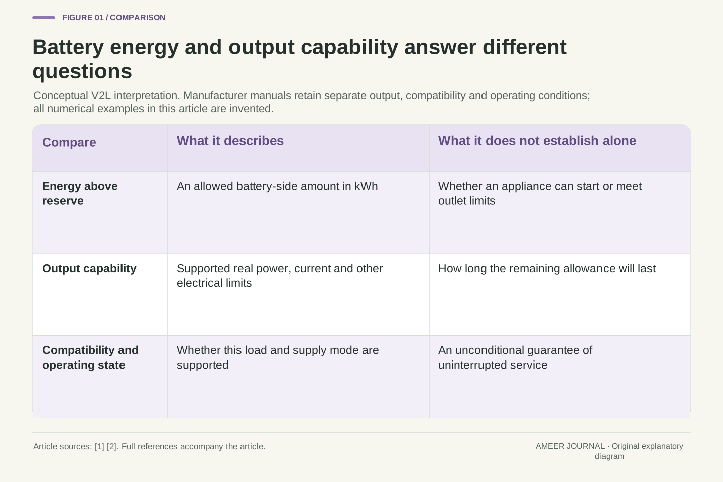
An ACC feature's presence in a vehicle does not mean it is providing the same support at every moment. Transport Canada notes manufacturer differences in operating range, while the Volvo page describes activation and availability conditions [1][5]. The selected settings, current indications and exact manual need to be read together. A remembered setting is not evidence that a function remains engaged after circumstances change.
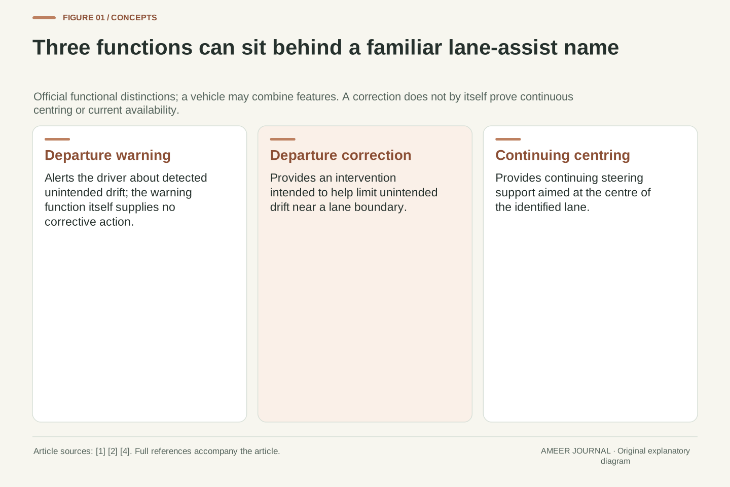
ACC also should not be confused with continual steering support or a separate emergency-braking function. NHTSA describes adaptive cruise, lane centering and automatic emergency braking as distinct technologies, and its driver-assistance descriptions retain the driver's active responsibility [2]. An ordinary slowing response while following traffic does not prove that an emergency intervention will occur in every later scene. The same distinction prevents a steering icon or a speed reference from being read as permission to stop monitoring the road. The driver must remain attentive and act when necessary under the applicable vehicle guidance.
Distinguish feature availability, a stored setting and current active support. The sources document varying operating ranges and activation conditions [1][5]; this article does not assert a universal three-state interface or color convention. A control-related display must be interpreted using its actual manual rather than inferred solely from an earlier successful following event.
Longitudinal following regulation, lateral centering and emergency collision mitigation have different purposes. NHTSA's functional definitions and driver-assistance descriptions support keeping them separate [2]. The presence of one does not establish the complete sensing, timing or actuation envelope of another. In particular, the piecewise braking example is not an AEB test, and the simple distance policy does not specify steering. A valid explanation retains the driver's responsibility and the supported system state while avoiding unsupported claims that assistance becomes independent driving merely because several functions operate together.
Read the definition before trusting the number
A useful explanation of an ACC display starts with the identity of each quantity. Is it the selected speed, actual speed, chosen interval, measured distance or a target-vehicle indication? If a time value is calculated, ask which speed is in its denominator. Our 40-metre example produced a two-second headway with no finite constant-speed contact time, an eight-second closing time, or an increasing gap, depending on the leader's motion.
Then ask what the number leaves out. Changing acceleration, target replacement, detection conditions and support state all matter. The original stopping example shows why a reasonable-looking snapshot cannot prove a future outcome, while the offset-policy example explains why a time coefficient need not equal observed gap divided by speed. Use those distinctions to read the exact vehicle documentation more carefully, not to shorten gaps or test system limits on the road. The value of the calculation is a better account of what is known, what was assumed and what the display alone cannot establish.
Keep the chain explicit: target and state identification, quantity definitions, relevant motion assumptions, and the scope of the resulting inference. H=d/vf and constant-velocity TTC=d/(vf−vl) use different denominators. The invented policy d_s+T vf adds another distinct quantity: a target distance whose ratio to speed need not equal T. None supplies a complete response envelope.
The worked cases expose different missing premises: unchanged relative motion, a stable target, a known braking trajectory and continuing support availability. Reusing a numerical result after changing one of those premises is not a valid prediction. The cited guidance supplies bounded descriptions of assistance, while the original calculations show how to interpret rather than inflate those descriptions. A careful reader can recognize that following support is useful without treating its selected interval as a collision countdown, a stopping-distance certificate or a substitute for attentive driving.
Sources & further reading
Explore the references behind this guide. External pages may change after our review.
- Adaptive cruise controlTransport Canada · Accessed 7 Nov 2026
- Driver Assistance Technologies | NHTSAU.S. National Highway Traffic Safety Administration · Accessed 7 Nov 2026
- Setting time interval to vehicle aheadPolestar · Accessed 7 Nov 2026
- 2.5 Motion Equations for Constant Acceleration in One Dimension - College Physics 2e | OpenStaxOpenStax / Rice University · Accessed 7 Nov 2026
- EX40 Adaptive cruise control conditions and limitations | Volvo Support HKVolvo Cars · Accessed 7 Nov 2026
Article updated 7 Nov 2026.
Found something we should revisit?
Good explanations get better with thoughtful feedback.