What you’ll take away
- PWM switching frequency, motor electrical frequency and shaft rotation describe different repeated events.
- A duty cycle controls a local average; instantaneous voltage, average and RMS remain different quantities.
- For the stated synchronous motor, mechanical rpm equals 60 times electrical frequency divided by pole pairs.
- Terminal differences and a specified modulation method determine how DC-link voltage constrains the motor fundamental.
- Torque and efficiency need current, operating-state and power-boundary information beyond a switching-rate number.
Fast electrical switches do not mean an equally fast rotor
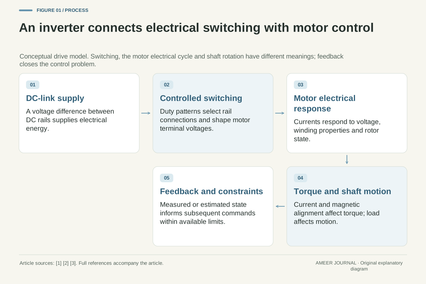
An electric motor controller can switch its power devices thousands of times each second while the motor shaft turns far more slowly. There is no contradiction. The fast switching helps create a controlled electrical waveform; the waveform's repeating motor cycle is a different rate, and shaft rotation is another. Analog Devices describes an inverter that synthesizes variable-frequency motor voltages from a DC supply using rapid switching [1]. Confusing the switching rate with the motor cycle skips the mechanism that connects them.
We will use a hypothetical two-level, three-phase inverter and a permanent-magnet synchronous motor. The model's battery-side DC link is 400 volts. Its illustrative switching frequency is 10 kHz, its motor electrical frequency is 100 Hz, and the motor has four pole pairs. These are invented teaching values, not a specification for any vehicle or instructions for operating power electronics. The question is how those quantities can coexist. Along the way, we will separate a pulse's instantaneous voltage from its average, a motor terminal difference from a voltage to a reference rail, and electrical output from mechanical output.
A PWM carrier, a motor's electrical fundamental and the rotor's mechanical frequency are distinct quantities. A voltage-source inverter uses semiconductor switching to synthesize controlled motor voltages from a DC link; the high-frequency switched waveform is not identical to its lower-frequency fundamental [1][2]. The carrier frequency therefore cannot be substituted directly into a rotor-speed relation.
The original examples use an ideal two-level three-phase bridge, a nominally constant 400 V DC link and a permanent-magnet synchronous motor for the electrical-to-mechanical speed relation. The illustrative frequencies are f_sw=10,000 Hz and f_e=100 Hz, with p=4 pole pairs. Numerical snapshots and operating comparisons are analytical, not hardware measurements. Ideal switching neglects finite transitions, device drops, dead time and parasitic paths until their relevance is discussed. No wiring, gate-drive implementation, calibration or power-stage access is proposed. The purpose is to identify the reference, averaging operation and physical boundary needed before a voltage or frequency number can support a claim about motor operation.
A duty cycle changes the average without changing the pulse height
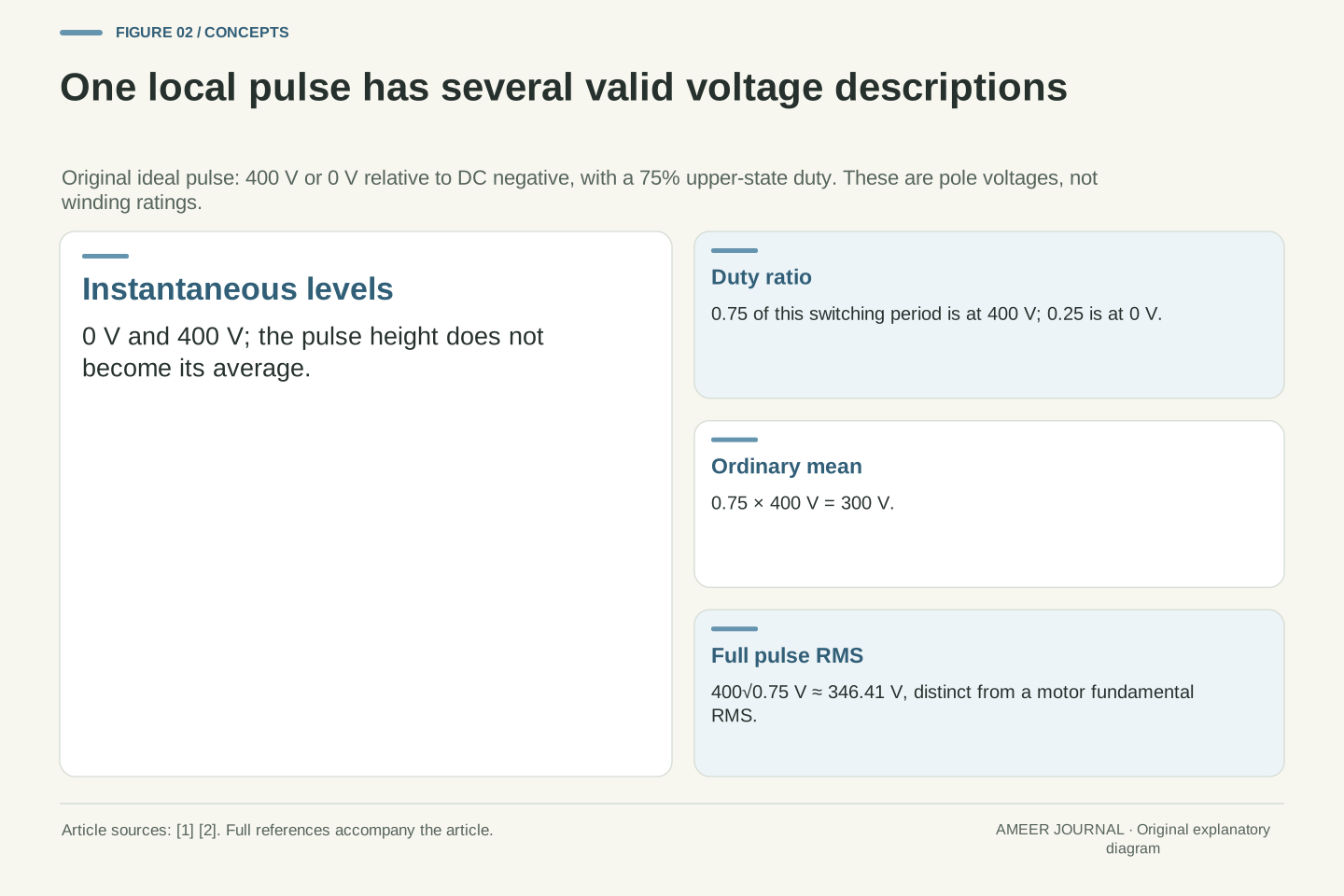
In the ideal model, one inverter output leg connects to either the positive DC rail or the negative rail. Measure its voltage relative to the negative rail: the two possible values are 400 V and 0 V. A duty cycle tells us what fraction of a short switching period is spent at the upper value. If that fraction is 75%, the average over the period is 0.75×400=300 V. The instantaneous output is still switching between the two rails; it does not become a steady 300-volt source. This averaging principle is central to PWM, or pulse-width modulation [1][2].
The kind of average also matters. For that same two-level pulse, the ordinary average is 300 V, while its root-mean-square value is about 346.41 V. Root-mean-square, shortened to RMS, squares the values, averages those squares and then takes a square root. Here that gives the square root of 0.75×400². These two results describe the same pulse in different ways. Neither is automatically the voltage across a motor winding: so far, we have described just one switching leg relative to the negative rail.
For one ideal leg referenced to DC negative, v_a0(t) takes values 0 and V_dc. If the upper-state fraction during a switching period is d_a, then its switching-period average is vbar_a0=d_a V_dc [2]. With V_dc=400 V and d_a=0.75, the average is 300 V. The duty ratio is held fixed within this local averaging example; a varying sequence of such duties can synthesize a changing low-frequency waveform.
The same local pulse has full-waveform RMS V_rms=V_dc√d_a=400√0.75 V≈346.410 V. Its mean is V_dc d_a=300 V. The RMS calculation includes the pulse's DC and switching components; it is not the RMS of a sinusoidal motor fundamental. Likewise, the 400 V pulse height does not equal a continuously applied 400 V winding voltage. Each value needs its reference nodes and time operation. These simple differences explain why a report can contain several valid voltages for one inverter while an unqualified comparison between them is misleading.
The duty pattern can change much more slowly than the switches
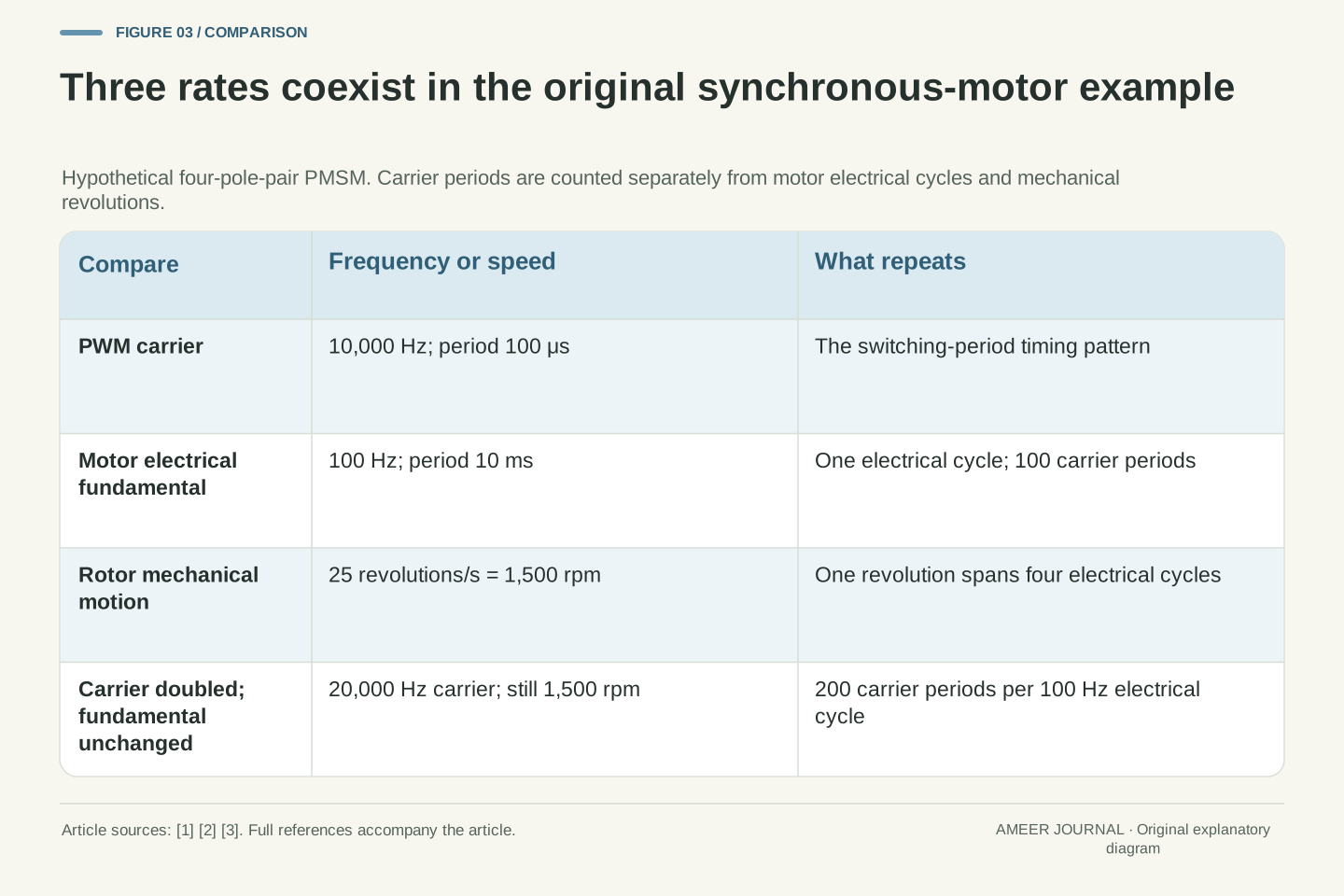
At a switching frequency of 10,000 cycles per second, one PWM period lasts 100 microseconds. A microsecond is one millionth of a second. The 100 Hz motor electrical waveform, meanwhile, repeats every 10 milliseconds. There are therefore 100 switching periods within one electrical cycle in this example. The controller can change the widths of many short pulses as it builds the slower pattern. Imperix's inverter explanation treats the sinusoidal modulation signal and the PWM carrier as separate parts of this process [2].
This is why doubling the switching frequency does not, by itself, double the motor's electrical frequency. If the slower pattern remains at 100 Hz while switching rises to 20 kHz, one electrical cycle now contains 200 switching periods. Its duration is still 10 milliseconds. Conversely, the slower pattern can change frequency while the switching rate stays fixed. The two rates are related by the controller's design and limits, but they describe different jobs. The pulse timing creates a controlled approximation to the desired waveform; the desired waveform does not acquire a new cycle each time a switch changes state.
The illustrative carrier period is T_sw=1/f_sw=100 μs. The electrical fundamental period is T_e=1/f_e=10 ms. Their ratio T_e/T_sw=f_sw/f_e=100 counts switching periods per electrical cycle. Carrier-based sinusoidal modulation compares the desired modulation signals with a carrier, while the resulting leg-voltage averages follow the lower-frequency references [2]. The count concerns periods, not a universal count of transistor transitions: actual edge counts depend on modulation and switching state.
At f_sw=20 kHz and unchanged f_e=100 Hz, the ratio becomes 200 while T_e stays 10 ms. This does not double synchronous rotor speed. Nor does a fixed 10 kHz carrier force the electrical fundamental to remain at 100 Hz. A real controller must accommodate sampling, computation, modulation and current response, but those implementation constraints do not make carrier frequency and electrical frequency identical [1][4]. The example separates their meanings without prescribing a particular ratio or claiming that every traction inverter operates at a constant carrier frequency.
Pole pairs connect the electrical cycle to shaft rotation
A permanent-magnet synchronous motor has magnetic pole pairs around its rotor. One mechanical revolution passes through as many electrical cycles as there are pole pairs. Microchip's motor-control documentation describes this distinction explicitly [3]. Our invented rotor has four pole pairs, so four electrical cycles correspond to one shaft revolution. At 100 electrical cycles per second, the shaft makes 100÷4=25 revolutions per second, or 1,500 revolutions per minute. The 10 kHz switching number is not part of that division.
The pole count must also be read correctly. Four pole pairs means eight individual poles. Substituting eight for four in the pole-pair formula would incorrectly halve the result. A separate synchronous motor with two pole pairs would rotate at 3,000 rpm at the same 100 Hz electrical frequency. These are kinematic relationships for the stated synchronous operation, not promises that a motor instantly reaches a requested speed. The car's road speed would additionally depend on its gearing and wheel geometry. Other motor types require their own relationship between rotor motion and electrical excitation.
For the stated PMSM synchronous relationship, θ_e=pθ_m and ω_e=pω_m, where p counts pole pairs [3]. Hence f_m=f_e/p and n_rpm=60 f_e/p. With p=4 and f_e=100 Hz, f_m=25 Hz and n=1,500 rpm. Using total pole count P=2p gives the equivalent n=120 f_e/P. These formulas agree only when the pole convention is kept consistent.
A two-pole-pair synchronous machine at the same f_e would have n=3,000 rpm. The example does not substitute inverter carrier frequency for f_e or claim that the shaft follows a frequency command without torque and dynamic constraints. It also does not apply the PMSM rotor-frequency equality indiscriminately to induction machines, where rotor motion relative to the rotating field needs separate treatment. Electrical frequency, shaft speed and vehicle speed occupy different stages of the interpretation. The conversion between the first two requires the appropriate machine relationship; the conversion to road speed requires the drivetrain and wheel information.
The motor sees differences between terminals, not a rail label alone
Take a separate switching-period snapshot with duties of 75%, 25% and 50% for legs a, b and c. Relative to the negative rail, their averages are 300, 100 and 200 V. The average voltage from terminal a to terminal b is the difference: 300−100=200 V. From b to c it is −100 V, and from c to a it is also −100 V. The signs record the order of the two terminals. A single leg's 300 V average is therefore not the same thing as the a-to-b voltage [2].
Now add 10 percentage points to all three duty values, keeping them within zero and one. The leg averages become 340, 140 and 240 V. Every pairwise difference stays unchanged. This shared shift is called a common-mode change. It illustrates why the reference matters, not why common-mode behaviour can always be ignored. Microchip notes that parasitic paths can make common-mode voltage physically significant [3]. Our arithmetic concerns the average terminal differences; it does not declare the DC negative rail, motor neutral or vehicle body to be the same electrical point.
For arbitrary leg averages relative to DC negative, vbar_ab=V_dc(d_a−d_b), and similarly for bc and ca [2]. At duties (0.75,0.25,0.50), the pole averages are (300,100,200) V and the line differences are (200,−100,−100) V. Their sum is zero, consistent with v_ab+v_bc+v_ca=0. No assumption that DC negative equals a motor neutral is needed for this pairwise identity.
Adding a common duty offset δ=0.10 gives duties (0.85,0.35,0.60), pole averages (340,140,240) V and unchanged line differences. The added δV_dc=40 V cancels in every subtraction. This is a local average-voltage example, not a complete switching sequence or a statement that all waveform details are unchanged. Common-mode voltage can couple through parasitic paths, including the effects discussed in the pinned Microchip documentation [3]. The relevant conclusion is narrower: a terminal-to-terminal quantity cannot be inferred from one pole voltage without its other terminal, and a reference-rail shift is distinct from a differential-voltage change.
The DC link limits the waveform that the duties can synthesize
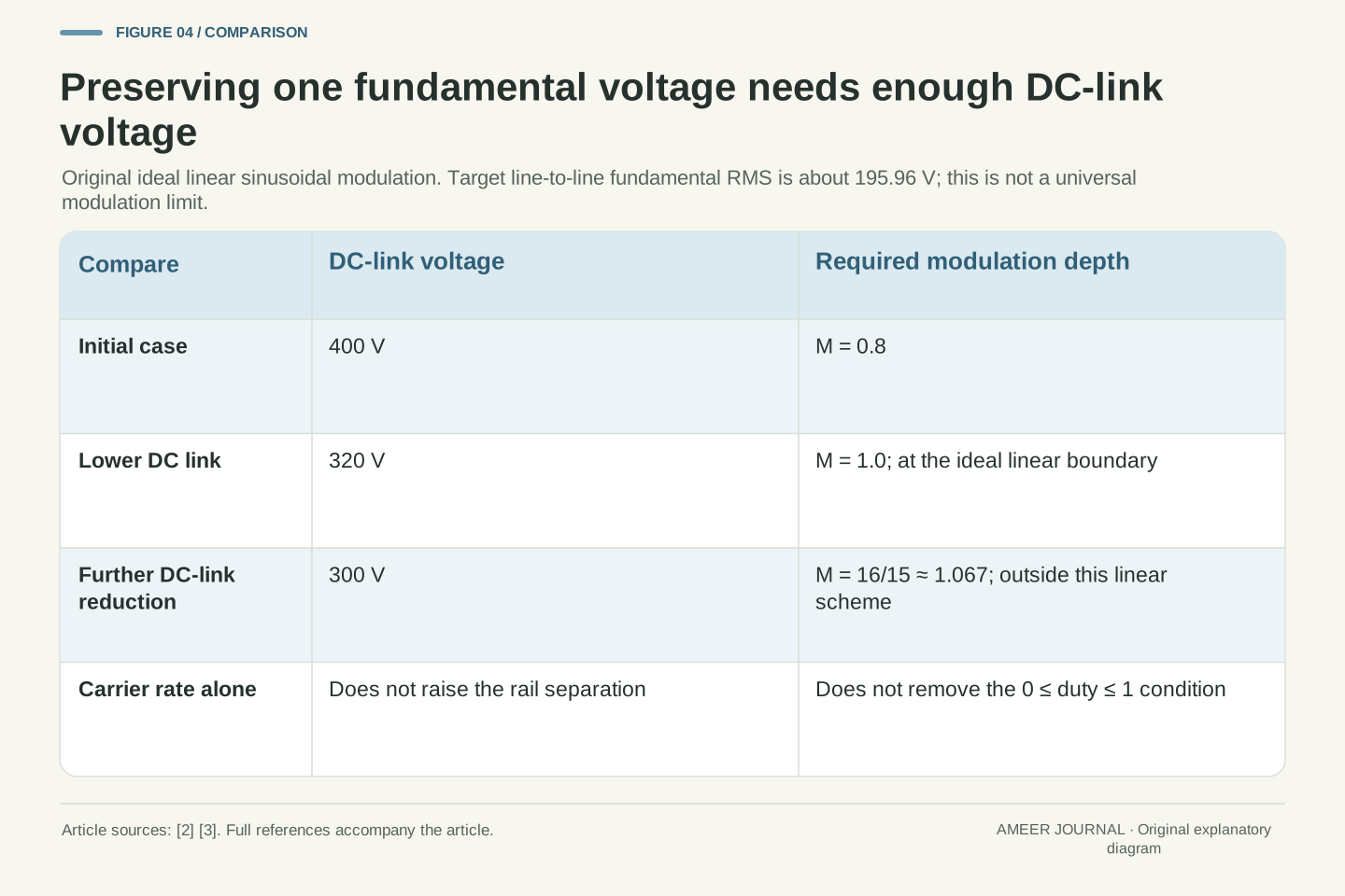
For a separate balanced sinusoidal example, use a modulation depth of 0.8. This describes how far the duty pattern swings around its halfway value; it is not an efficiency. In the ideal sinusoidal scheme, a 400 V DC link then gives a phase-to-neutral fundamental peak of 160 V. The corresponding fundamental line-to-line RMS voltage is about 195.96 V. Imperix derives the relationships between modulation, phase voltage and line-to-line voltage for its stated inverter model [2]. Peak, RMS, phase-to-neutral and line-to-line remain different labels.
Suppose the DC link falls to 320 V while the same modulation depth is retained. The line-to-line fundamental RMS falls to about 156.77 V. Restoring the earlier 195.96 V would require increasing the depth from 0.8 to 1.0. At a 300 V link, it would require about 1.067, beyond the zero-to-one duty limits of this simple linear sinusoidal scheme. This does not set a universal ceiling for every modulation strategy. It shows why the controller cannot ask this particular scheme for an arbitrary voltage merely by choosing a faster switching rate.
For balanced sinusoidal modulation, d_i=(1+M sin θ_i)/2 with the phase angles separated by 120°. In the ideal linear range 0≤M≤1, the fundamental phase-to-neutral peak is M V_dc/2, and fundamental line-to-line RMS is √3 M V_dc/(2√2) [2]. At M=0.8 and V_dc=400 V, these are 160 V and approximately 195.959 V. The RMS relation applies to the sinusoidal fundamental, not the complete switched pole waveform calculated earlier.
At V_dc=320 V with M fixed, the line RMS becomes approximately 156.767 V. Preserving the original fundamental requires M_new=M_old V_old/V_new: 1.0 at 320 V and 16/15≈1.0667 at 300 V. The latter would require some duties outside [0,1] in this sinusoidal linear model. Other modulation methods can use the DC bus differently, so the calculation is not a universal inverter voltage-utilization limit. Even at M=1 the ideal example has no modulation margin. Changing carrier frequency alone does not increase the available rail separation or remove the duty constraints.
A voltage pattern still needs a current-control problem to solve
Producing a voltage pattern is not the same as producing a particular torque. Motor current responds to voltage, winding properties and the motor's electrical state. Its relationship to the rotor's magnetic field matters as well. Microchip explains field-oriented control as management of current components relative to a rotating reference, while Analog Devices describes feedback from motor currents and rotor position or its estimate [1][3]. The inverter is part of that control system, not a device that reads one speed number and automatically supplies whatever torque is needed.
This explains two everyday-looking situations without giving them identical causes. A motor can turn at the same speed while providing different torque to meet different loads. It can also need torque while its speed is changing. The electrical frequency-to-speed relationship does not specify how much current is required in either case. Current limits, voltage availability and thermal constraints can restrict what the drive can provide. A useful inverter description therefore keeps commanded behaviour, measured or estimated state and available capability separate. Faster switching cannot substitute for missing information about the load or for the current and voltage needed to control it.
For the PMSM case, torque depends on current and flux alignment rather than electrical frequency alone. The pinned Microchip account expresses electromagnetic torque through the cross product of flux linkage and current and describes inner current control with an outer velocity loop [3]. Analog Devices likewise separates current regulation, voltage synthesis and measured or estimated rotor state [1]. The article does not assume that every drive uses one identical controller or position sensor.
A realizable voltage command must drive the required current response while respecting available DC-link voltage and other constraints. The source discussion explicitly notes that changing current requires voltage through inductive terms and that on-state drops and dead time reduce idealized margin [3]. Torque demand also depends on the external load and desired acceleration. Equal rotor speed therefore need not imply equal current, torque or power. The synchronous speed relation is a coordinate and machine relationship, not a complete dynamic model. Treating it as one would conceal the very feedback and limiting functions that make controlled motor operation possible.
More switching can reduce ripple while adding another cost
A motor winding's inductance resists rapid changes in current. That helps explain how a rapidly pulsed voltage can produce a smoother current waveform rather than an equally sharp sequence of current pulses [1]. In a simple local calculation, assume 20 V acts across an ideal 1 millihenry inductance for 10 microseconds. The current changes by 0.2 A. If the same voltage acts for only 5 microseconds, the change is 0.1 A. The shorter interval allows less change; this is a deliberately simplified illustration of ripple, not a complete motor model.
That benefit does not make an arbitrarily high switching frequency the best choice. Real switches incur losses while conducting and during transitions. TI discusses this trade-off when explaining higher-frequency motor drives [4]. Device characteristics, the operating point, cooling and the modulation pattern all affect the result. Increasing switching frequency can give a controller more opportunities to shape the waveform, but it does not automatically improve the efficiency of the complete drive. It also does not change the pole-pair conversion between a given motor electrical frequency and shaft speed. Those questions remain separate even when one design choice influences several of them.
For a local ideal inductance, Δi=V_L Δt/L when V_L is constant over the interval. With V_L=20 V, L=1 mH and Δt=10 μs, Δi=0.2 A; halving the interval gives 0.1 A. This original interval calculation illustrates the connection between switching timescale and ripple under fixed conditions. A complete winding model also includes resistance, induced voltage, changing state and the actual switching sequence [1][3]. It does not follow that every real ripple value scales exactly with the carrier ratio.
The trade-off includes semiconductor conduction and switching losses. TI's technical discussion uses this distinction to explain why simply raising switching frequency is not a free improvement [4]. An approximate switching-loss account would need energy per transition and the number and type of transitions, all at defined operating conditions. This article supplies no universal loss coefficient or present device ranking. Control bandwidth, pulse resolution, thermal constraints and current ripple need to be assessed together. None changes the meaning of f_e or p in the synchronous rotor-speed relation; a carrier change affects the implementation, not the definition of a mechanical revolution.
Inverter output is electrical power, not yet shaft power
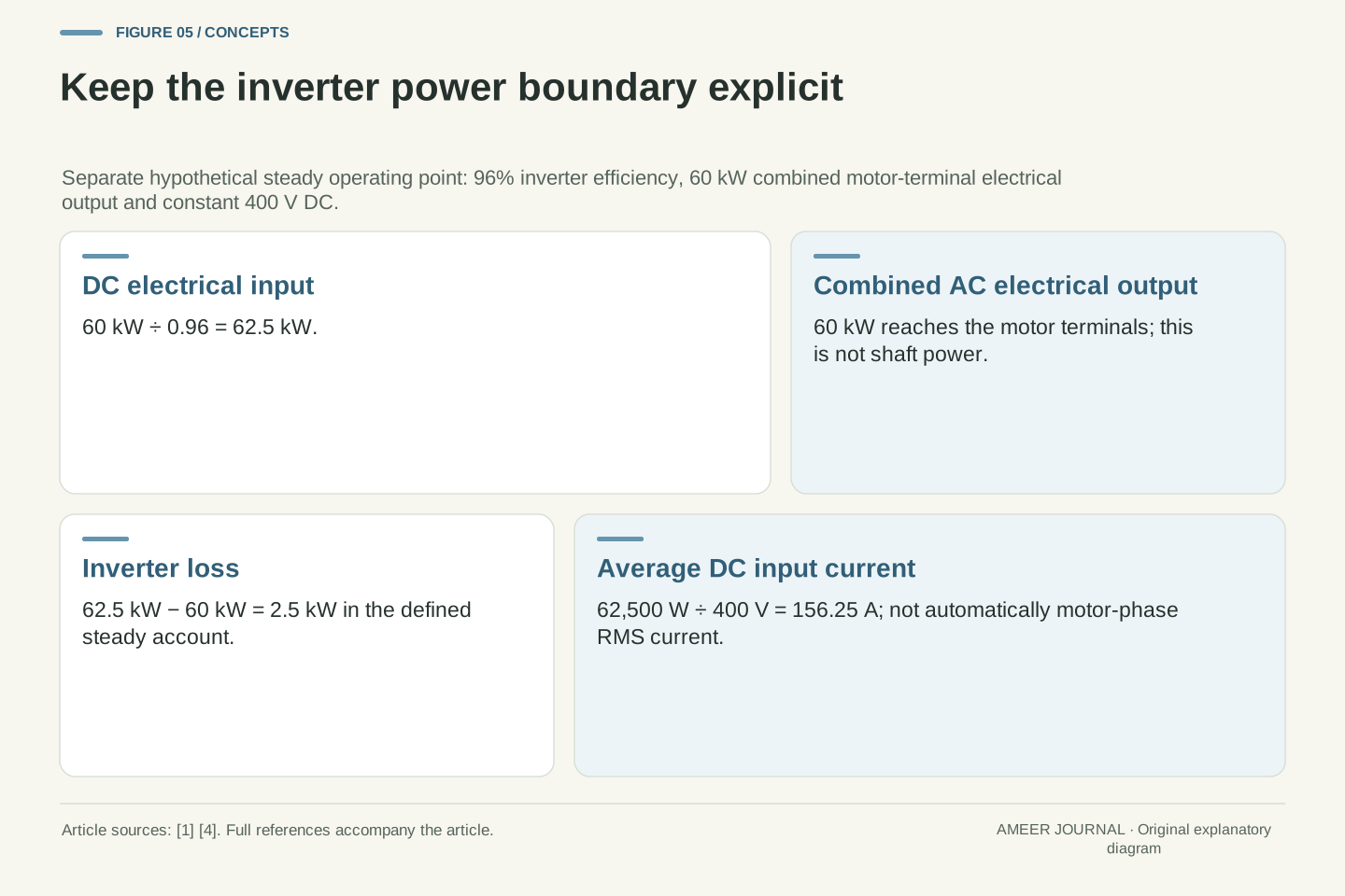
Consider another hypothetical operating point: 60 kW of electrical power reaches the motor terminals, and the inverter efficiency is assumed to be 96%. The DC input must then be 60÷0.96=62.5 kW. The difference, 2.5 kW, is inverter loss in this steady account. At a constant 400 V DC input, 62,500÷400 gives an average input current of 156.25 A. These numbers are internally consistent assumptions, not a measured inverter efficiency or a rating for the earlier waveform example.
The 60 kW is still electrical output. Finding mechanical shaft power requires the motor's losses and operating state as well. Likewise, the 156.25 A DC input is not automatically the RMS current in each motor phase. The motor side has multiple changing voltages and currents; its power must be accounted for across those terminals. The source descriptions distinguish DC conversion, motor current regulation and semiconductor losses [1][4]. A comparison that labels every one of these quantities simply 'motor power' can hide where the losses or measurements belong. Naming the boundary keeps an efficiency percentage interpretable.
At a separate stipulated steady operating point, define inverter efficiency as η_inv=P_ac/P_dc=0.96 and real three-phase electrical output P_ac=60 kW. Then P_dc=62.5 kW and P_loss=P_dc−P_ac=2.5 kW, with no changing stored-energy term in this account. At constant DC-link voltage 400 V, average I_dc=P_dc/V_dc=156.25 A. If DC voltage were varying materially, power would require averaging the instantaneous voltage-current product rather than multiplying arbitrary averages.
P_ac is the combined electrical power delivered to the motor terminals, not shaft power and not the power of one phase. A complete conversion chain would retain the motor's electrical and mechanical losses separately. Neither the inverter efficiency nor average DC current determines a phase RMS current without the relevant waveform and load information. The cited descriptions of PWM motor control and semiconductor loss support these distinct boundaries [1][4]; the 96% value is purely an input to our example. It is not attributed to those sources, treated as constant across operating points, or used to claim a real vehicle range benefit.
A voltage figure needs its nodes and its time definition
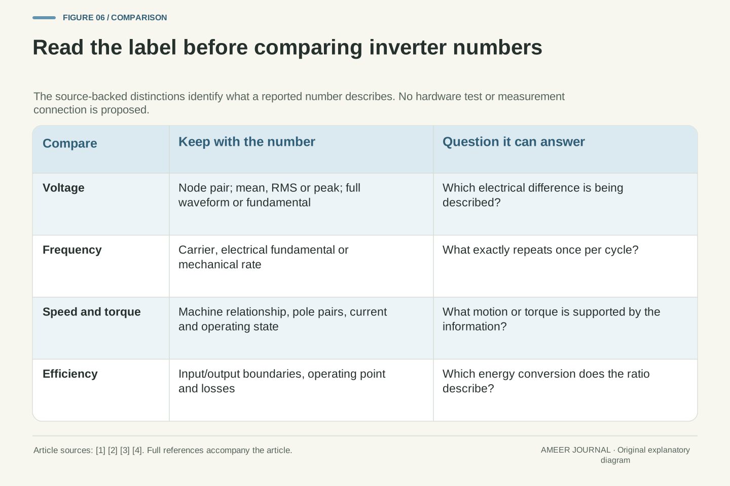
The earlier examples produced 400 V, 300 V, 346.41 V, 160 V and 195.96 V without any arithmetic conflict. They did not all describe the same thing. The first was a DC rail separation; the next two were the mean and RMS of one local pole pulse; the final two described a sinusoidal fundamental with different voltage references and peak/RMS conventions. A number becomes useful when the label says which of those questions it answers [2][3].
The same care applies to a waveform picture. A smooth drawn sine wave may represent the desired fundamental rather than the actual instantaneous terminal voltage. A jagged switched-voltage trace does not prove that the current has the same shape, because the winding's response matters [1]. When reading a report, ask whether it shows a command, an averaged model or a measured signal, and whether the voltage is pole-to-rail, phase-to-neutral or line-to-line. These are interpretation questions. No measurement method, probe connection or access to a vehicle's high-voltage system is needed to understand why the labels change the meaning.
Voltage interpretation requires both a node pair and a mathematical operation. V_dc, a switching-period pole mean, a full switched-waveform RMS, a phase fundamental peak and a line fundamental RMS are different quantities. Microchip explicitly warns that motor voltage-related constants can be ambiguous about peak versus RMS and line-to-line versus line-to-neutral conventions [3]. The same dimensional discipline is needed when reading inverter descriptions.
In particular, the 346.410 V RMS of the local 75% pole pulse cannot replace the 195.959 V line fundamental RMS of the separate M=0.8 sinusoidal example. The values use different waveforms, references and averaging windows. Nor does a fundamental-only model reproduce every switching harmonic, common-mode effect or current transient. The source inverter derivation clearly separates the switched waveform from the considered fundamental [2]. A good comparison preserves these labels and states whether evidence is simulated, measured or an ideal calculation. It should not infer a complete waveform or a hardware capability from a lone RMS number.
Connect the numbers only after naming their different jobs
Return to the hypothetical 10 kHz inverter and 100 Hz motor electrical cycle. At four pole pairs, the synchronous rotor turns at 1,500 rpm. Increasing the carrier to 20 kHz while retaining the same electrical cycle does not change that speed relation. It changes how the controller can construct the waveform, with consequences that require a separate ripple, loss and control analysis. The distinction is physical, not just a matter of using different units.
A useful description therefore names the DC supply, the switched and fundamental voltages, the carrier rate, the electrical frequency and the motor relationship. If it also claims torque or efficiency, it needs the current/state information and a defined power boundary. Our average-voltage, pole-difference, modulation-limit and power-ledger examples show what each additional input contributes. The inverter connects these parts of the system through controlled switching [1][2][3]. Reading them separately first makes it possible to connect them correctly, instead of turning one impressive frequency or voltage into a promise about shaft speed, torque or vehicle performance.
The worked interpretation starts with f_sw=10 kHz, f_e=100 Hz and p=4, giving 100 carrier periods per electrical cycle and n=1,500 rpm for the specified PMSM relationship. A 20 kHz carrier gives 200 periods without changing n if f_e and p remain fixed. The voltage examples independently establish vbar_a0=d_a V_dc, vbar_ab=V_dc(d_a−d_b) and the stated sinusoidal fundamental limit. These relations answer different questions and cannot replace one another.
Finally, the separate steady power example keeps DC input, combined AC electrical output and inverter loss at 62.5, 60 and 2.5 kW. Motor shaft output would require further information. A defensible inverter claim retains its operating point, modulation method, machine type, reference nodes and measurement definition [1][2][3][4]. The result is not a universal controller prescription. It is a practical way to determine whether the available evidence supports a statement about switching, electrical excitation, mechanical speed, torque or efficiency—and to identify the missing information when it does not.
Sources & further reading
Explore the references behind this guide. External pages may change after our review.
- Fundamentals of DSP-Based Control for AC Machines | Analog DevicesAnalog Devices · Accessed 6 Nov 2026
- Voltage source inverter - control software example - imperixImperix · Accessed 6 Nov 2026
- 5.1.1. Introduction — MCAF R6 RC8 documentation (docver 6.0.2)Microchip Technology · Accessed 6 Nov 2026
- SSZTAJ4 Technical article | TI.comTexas Instruments · Accessed 6 Nov 2026
Article updated 7 Nov 2026.
Found something we should revisit?
Good explanations get better with thoughtful feedback.