What you’ll take away
- Single-speed means one available overall ratio, not one road speed or no transmission.
- A reduction trades lower output speed for higher output torque; ideal gearing conserves mechanical power.
- Always identify the shaft and loss boundary before comparing torque or efficiency numbers.
- A motor’s torque-speed envelope determines whether a calculated wheel output is actually available.
- A motor-rpm ceiling is a kinematic constraint, not evidence of an achieved vehicle top speed.
Single-speed describes a ratio, not one road speed
An electric car can have a transmission even when the driver never selects a numbered gear. The US Department of Energy lists the transmission as the component that transfers mechanical power from the traction motor to the wheels. [1] In a single-speed drive, one fixed reduction ratio connects the motor's rotation to the driven wheels. That does not mean the car travels at one speed, or that its motor and wheels turn equally fast. The motor can change speed while the same ratio remains engaged.
This article follows one imaginary motor-to-wheel path. It asks what the ratio changes, what it cannot create, and which missing facts prevent a gear specification from becoming an acceleration prediction. All numerical values are invented, and the calculations are not measurements of a vehicle. We will also distinguish one ratio from one physical gear pair: several fixed stages can form a single overall reduction. The underlying gear relationships apply to each stage and can be combined. [2][4] No driving experiment, software adjustment or mechanical modification is needed to understand the results.
A single-speed electric drive can contain a mechanical transmission with one available overall reduction ratio. The DOE component description explicitly places an electric transmission between the traction motor and the driven wheels. [1] Fixed ratio does not imply equal shaft speeds, a constant vehicle speed, or a constant commanded torque. It specifies a kinematic relationship while the motor operates across a range of speeds and torques.
Use one hypothetical forward-driving path with a motor shaft and an equivalent driven-wheel output. The wheel-output quantities describe that path's combined output, not the torque at every individual wheel or the sum of unrelated motor specifications. Straight rolling with equal wheel speeds is assumed; differential action and tyre slip are outside the model. Multiple fixed stages can be represented by their product ratio. [2][4] The following calculations are algebraic examples, not a vehicle simulation or measured performance map. They are intended to separate gearing, torque, power and operating limits before interpreting a real specification.
Write down which shaft is in the numerator
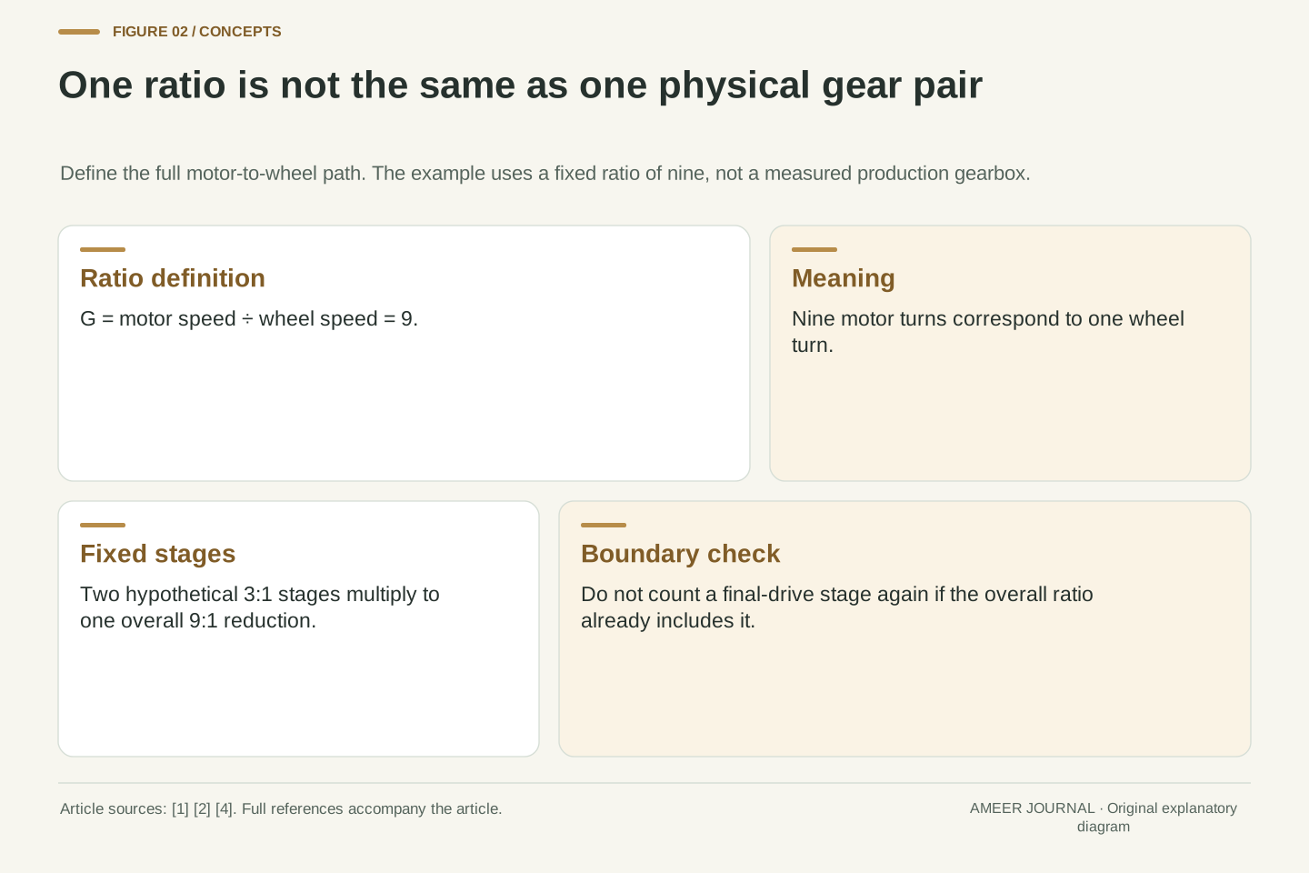
Define our reduction ratio as motor speed divided by wheel speed. A ratio of nine means nine motor turns for one wheel turn. If the motor makes 4,800 revolutions each minute, the wheels make 4,800 divided by nine: about 533.3 revolutions per minute. Mechanical references sometimes name their ratios differently, so a bare number such as nine is less useful than a sentence identifying both shafts. The reciprocal speed and torque relationships follow from the geometry of meshing ideal gears. [2]
The word overall matters. Suppose one fixed stage reduces speed three to one, and another reduces it three to one again. Together they produce nine to one, even though neither stage alone has that ratio. Northwestern's engineering teaching material describes this multiplication of consecutive gearbox ratios. [4] Counting visible gears would therefore answer a different question from counting the selectable ratios. Likewise, a final-drive ratio and a gearbox ratio must not be accidentally counted twice if a published overall number already includes both. The useful starting point is the entire path from the specified motor shaft to the road wheels.
Define G = ωm/ωw using positive speed magnitudes in this forward-drive example. Thus ωw = ωm/G. Let G = 9 for the baseline, so a motor speed nm = 4,800 rpm gives nw = 533.333 rpm. Individual meshing gears can rotate in opposite directions; this scalar reduction convention deliberately omits their internal direction changes. MathWorks distinguishes these sign conventions while showing that the magnitude of the speed ratio is reciprocal to the torque ratio for ideal gearing. [2]
For consecutive fixed stages G1 and G2, the overall reduction is G = G1G2. Two hypothetical 3:1 stages therefore give a 9:1 path. [4] This is a statement about ratio composition, not a declaration that every EV uses that architecture. A quoted component ratio may already incorporate other stages, and a wheel-output ratio must refer to the same shaft boundary as the torque figures being compared. Establishing that boundary first avoids apparent contradictions caused by treating a motor torque, an intermediate-shaft torque and a combined wheel torque as if they were measured at one location.
The controller changes output without changing the gears
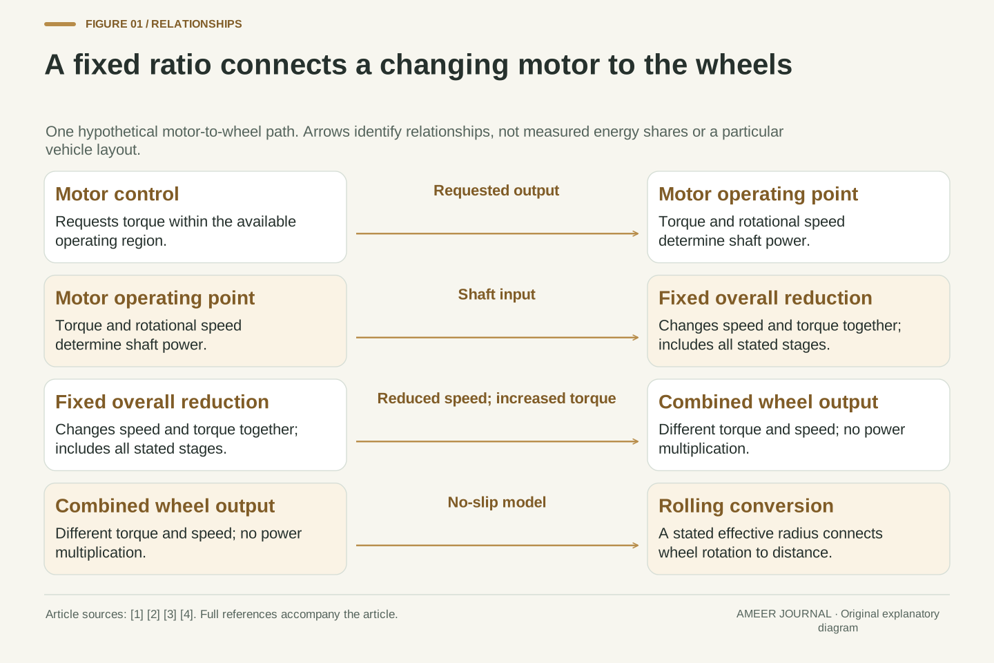
A fixed gearbox does not decide how much torque the motor must produce at every moment. DOE describes the power-electronics controller as managing energy flow and controlling the traction motor's speed and torque. [1] Asking for less wheel effort can therefore mean less motor torque through the same ratio. It does not require a different mechanical gear each time the driver eases the accelerator. Road speed changes as the vehicle responds to the forces acting on it, while the motor and wheel rotation remain connected by the fixed reduction.
There are limits to what can be requested. A useful engineering model has a permitted region of torque and speed rather than one torque number valid everywhere. MathWorks' generic motor-and-drive model applies such a region to a requested torque. [3] That source describes a model, not a test of a particular car. Its useful lesson is the distinction between a request and an available output. To judge a real drive, we would need the appropriate motor and controller limits under the relevant conditions. A single headline peak does not supply that entire operating picture.
The transmission's kinematic constraint and the controller's torque command are separate descriptions. DOE identifies the power-electronics controller as managing traction energy flow and motor torque/speed. [1] With G fixed, changing requested torque changes the output torque through the same mechanical ratio. The ratio alone supplies neither the command nor the available electrical power, and it does not prescribe a vehicle acceleration independently of the external loads.
MathWorks' generic Motor & Drive block illustrates this separation: a closed-loop torque request is constrained by a torque-speed envelope, with maximum torque and maximum power defining the boundary. [3] It is explicitly a simplified model. We use it as a framework for interpreting an envelope, not as evidence of any manufacturer's actual torque curve or control response. A real operating-point claim requires applicable limits and conditions, including whether the stated output is sustainable for the required duration. Fixed gearing can connect many operating points; it does not make every point physically available merely because the controller could request it.
Turn wheel rotation into distance, using a stated radius
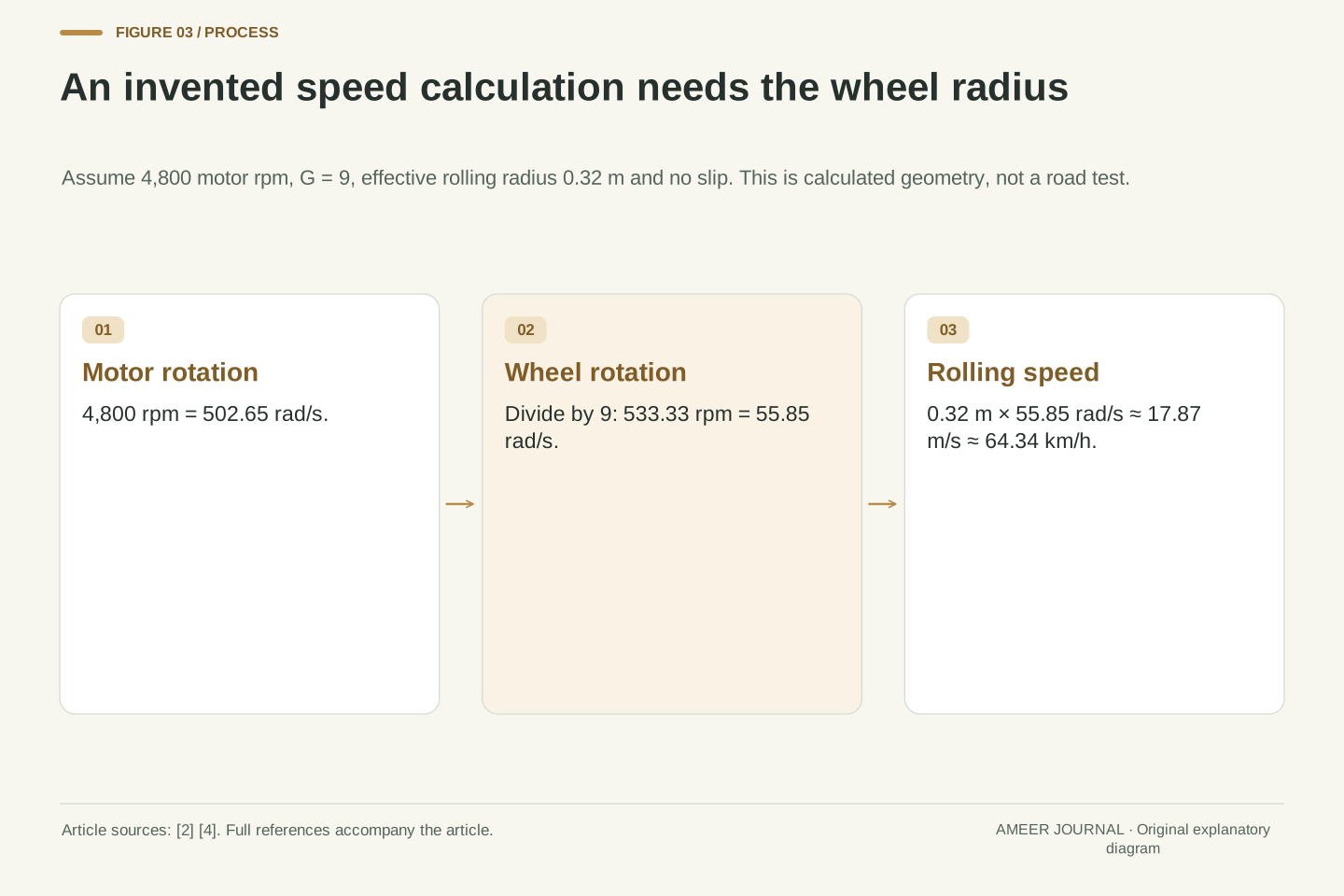
Give the imaginary driven wheels an effective rolling radius of 0.32 metres. One turn then covers roughly 2.01 metres, because a circle's circumference is twice pi times its radius. At 533.3 turns per minute, the corresponding road speed is about 17.87 metres per second, or 64.34 kilometres per hour. This completes the speed calculation from 4,800 motor rpm through the nine-to-one reduction. The result belongs to the assumed rolling radius and no-slip model; it is not a road test or a suggested speed.
Changing the assumed wheel radius would change this road-speed result even if the motor speed and reduction stayed identical. That is why a motor-rpm number and a gearbox ratio alone do not fully specify vehicle speed. The example uses the distance travelled per wheel turn, not a measurement taken from a photograph of a tyre. Real technical comparisons need compatible definitions for wheel rotation and rolling distance. We also assume the wheels are moving together in a straight line. A diagram of one equivalent output is not an account of every wheel's motion during a turn.
Let r = 0.32 m be a hypothetical effective rolling radius, with no longitudinal slip. Then ωm = 4,800 × 2π/60 = 502.6548 rad/s and ωw = ωm/9 = 55.8505 rad/s. The rolling constraint gives v = rωw = 17.8722 m/s, equivalent to 64.3398 km/h. These values are kinematic consequences of the chosen ratio and radius, not measured speeds. The radians-per-second conversion is essential when connecting rotational quantities to SI power and linear velocity.
Alternatively, circumference 2πr = 2.0106 m multiplied by 533.333 wheel revolutions per minute gives the same distance per minute. This independent route checks the rpm conversion. The effective radius is a modelling assumption tied to rolling distance, not an assertion about unloaded tyre dimensions or behaviour under slip. For a fixed motor speed and ratio, the model's linear speed scales with r. Consequently, a numerical rpm-to-road-speed statement must expose its radius assumption. Internal gear geometry determines the shaft ratio; wheel-road geometry supplies a separate conversion at the output.
More wheel torque does not mean more power
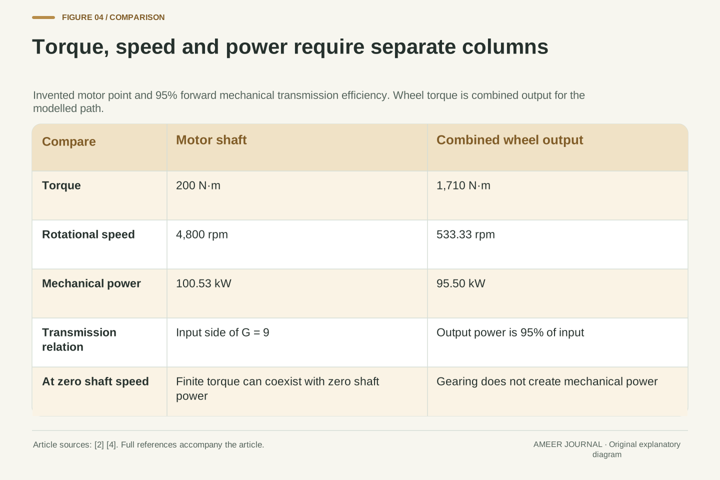
Now let the motor deliver an invented 200 newton-metres of torque at those 4,800 rpm. An ideal nine-to-one reduction would provide 1,800 newton-metres at the combined wheel output while turning nine times more slowly. The ideal gearbox trades rotation speed for torque; it does not multiply both together. Their product is mechanical power. MathWorks and Northwestern explain this conservation across an ideal gear coupling. [2][4] The output torque is larger because each output turn takes more input turns, not because the gearbox supplies extra energy.
Add an assumed 95 percent forward transmission efficiency. The combined wheel torque becomes 0.95 × 9 × 200 = 1,710 newton-metres. Motor-shaft power is about 100.53 kW; wheel-output power is about 95.50 kW. The difference, roughly 5.03 kW, is the model's transmission loss. These are mechanical powers at two shaft boundaries. Battery power would also need the motor, electronics and other electrical loads. The 95 percent figure is an invented constant for this calculation, not a measured gearbox rating or a claim that efficiency stays fixed at every operating point. [4]
For ideal gearing, Tw = GTm while ωw = ωm/G, so Pw = Twωw = Tmωm = Pm. The torque gain cancels the angular-speed reduction in the power product. [2] With Tm = 200 N·m and ωm = 502.6548 rad/s, Pm = 100.5310 kW. An ideal G = 9 gives Tw = 1,800 N·m. Neither the numerical torque multiplication nor its unit denotes an energy multiplication.
Introduce a stipulated forward efficiency ηg = 0.95. For this positive power flow, Tw = ηgGTm = 1,710 N·m and Pw = ηgPm = 95.5044 kW; the difference is 5.0265 kW. Northwestern derives this same relationship for a nonideal transmission that preserves the speed constraint while reducing delivered torque and power. [4] This ηg belongs solely to the defined mechanical transmission boundary. It is not battery-to-wheel efficiency, a reverse-flow efficiency or a constant inferred for a real product. Calculating battery input would require additional conversion losses and loads, with consistent boundaries to prevent double counting.
At zero speed, torque and power tell different stories
The same power relationship explains a statement that often sounds contradictory: a motor can produce torque while its shaft has zero rotational speed, yet its mechanical shaft power at that instant is zero. Power equals torque multiplied by rotational speed. [2] The gearbox can multiply the available torque, but it cannot turn zero shaft motion into positive output mechanical power. As the vehicle begins moving, the same torque corresponds to increasing mechanical power because the shaft is now rotating.
Zero mechanical output power does not prove zero electrical input or zero heating. The motor-and-drive model explicitly separates electrical input, mechanical output and losses. [3] It is therefore wrong to read a motor's peak kilowatt figure as power delivered at every speed, including standstill. This distinction is a way to read specifications, not an instruction to hold a real vehicle against its brakes or test stall behaviour. The actual available launch torque, duration and control behaviour need vehicle-specific evidence; neither our ratio nor the zero-speed identity establishes them.
At ωm = 0, the shaft power Pm = Tmωm is zero for any finite Tm. The kinematic relation also makes ωw zero, so Pw is zero. [2] A nonzero torque remains meaningful: it describes rotational effort at that instant, while mechanical power describes the rate of work through angular displacement. The limit is especially useful when interpreting claims that conflate an available launch torque with maximum mechanical kilowatts.
This identity does not set electrical input to zero. MathWorks' motor model writes electrical power as mechanical output plus losses and separately represents torque-related resistive loss. [3] Its simplified loss law is not a complete traction-motor thermal model, so we do not calculate a stall current, temperature rise or safe holding duration from it. Similarly, the constant transmission efficiency used at the moving example should not be treated as a measured zero-speed efficiency. The rigorous conclusion is narrower: torque may be nonzero while shaft work rate is zero, and an electrical energy balance remains a separate question.
Compare two reductions at the same road speed
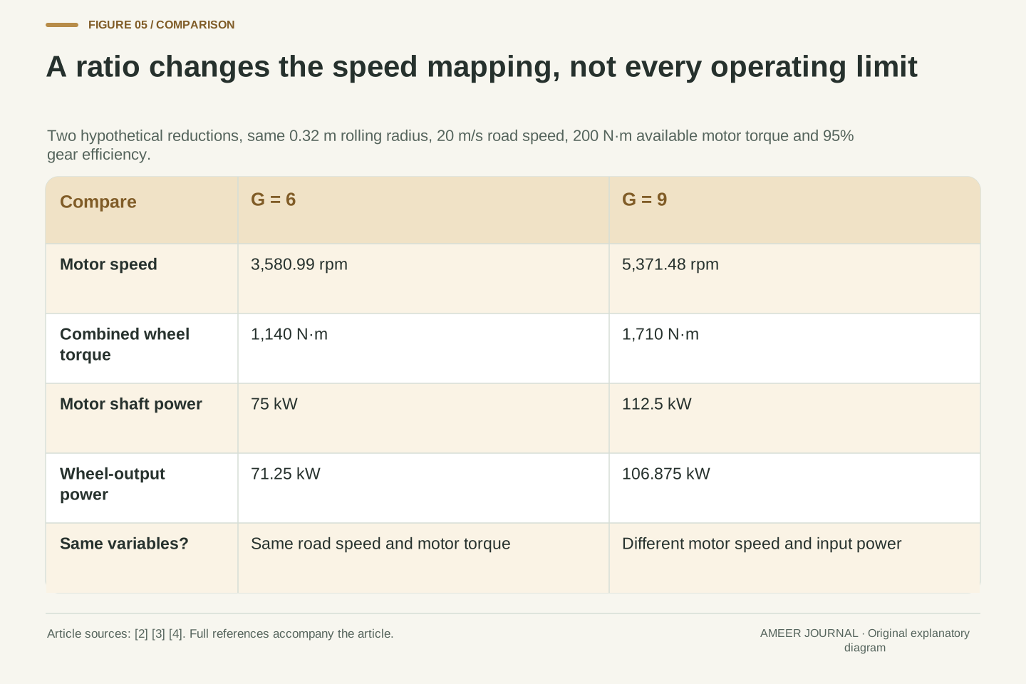
Keep the imaginary radius at 0.32 metres and choose a road speed of 20 metres per second. A nine-to-one reduction now requires about 5,371 motor rpm. A six-to-one reduction requires about 3,581 rpm. Assume, for this comparison only, that the motor can provide 200 newton-metres at either operating point and that transmission efficiency remains 95 percent. The combined wheel torques are then 1,710 and 1,140 newton-metres respectively. The larger reduction provides more wheel torque but asks the motor to turn faster at that same road speed.
This is not free extra performance from one unchanged motor operating point. The two cases use different motor speeds, so the same motor torque corresponds to different mechanical powers. Whether both points are available depends on the motor's operating envelope. [3][4] And a wheel-torque comparison is not yet a timed acceleration result: tyre contact, vehicle mass, resistance and rotating components also matter. Northwestern's discussion explicitly notes that some mechanical power accelerates the rotor itself. [4] The calculation isolates the ratio trade-off; it does not predict a complete vehicle's launch time or traction on a road.
At v = 20 m/s and r = 0.32 m, ωw = v/r = 62.5 rad/s. G = 9 requires ωm = 562.5 rad/s, or 5,371.48 rpm; G = 6 requires 375 rad/s, or 3,580.99 rpm. Stipulating Tm = 200 N·m and ηg = 0.95 at both points gives Tw = 1,710 versus 1,140 N·m. The corresponding motor mechanical powers are 112.5 and 75 kW, with output powers 106.875 and 71.25 kW.
Thus this is an equal-road-speed, equal-motor-torque comparison, not an equal-input-power comparison. The higher-reduction case draws more mechanical power from the motor because its shaft rotates faster. Both points must lie within the applicable torque-speed envelope before their calculated outputs can be considered available. [3][4] Converting torque into vehicle acceleration would additionally require a contact-force and inertia model, including losses and external resistance. The present equivalent shaft model does not supply those details. Its valid result is the conditional trade between shaft speed and wheel torque, without a predicted acceleration time.
A constant-power region gives a different answer
Build a deliberately simple imaginary motor envelope. Allow 200 newton-metres up to 6,000 rpm, then hold its maximum mechanical power constant while speed rises toward 12,000 rpm. At 6,000 rpm, 200 newton-metres corresponds to about 125.66 kW. At twice that speed, keeping the same power requires half the torque: 100 newton-metres. This invented envelope follows the torque-and-power boundary idea used in the MathWorks model; it is not a measured curve or a promise about any particular EV. [3]
With our nine-to-one reduction and 95 percent efficiency, the combined wheel torque is 1,710 newton-metres at the first point and 855 at the second. Output speed doubles, so output mechanical power stays about 119.38 kW. Now suppose two different reductions place the motor inside the same constant-power region at one chosen road speed. If they deliver the same shaft power and have equal transmission efficiency, their wheel powers—and therefore their wheel torques at that common wheel speed—are equal. A larger ratio cannot create an automatic torque advantage after the assumed motor torque has already fallen to preserve power.
Define an illustrative envelope with Tmax = 200 N·m through nb = 6,000 rpm and Pmax = Tmax × 2πnb/60 = 125.6637 kW above that point, up to an imposed 12,000 rpm model boundary. This is an original piecewise assumption, using the maximum-torque/maximum-power envelope concept described by MathWorks. [3] At 12,000 rpm, T = Pmax/ω = 100 N·m. No measured efficiency map, field-weakening law or real continuous rating is implied.
For G = 9 and ηg = 0.95, those boundary points produce Tw = 1,710 and 855 N·m respectively, while Pw = 119.3805 kW at both. More generally, when two ratios at the same ωw both place the motor in a common constant-power region, Tw = ηgPmax/ωw if efficiencies are equal. The ratio cancels from this expression because the motor torque adjusts inversely with its speed. That conditional cancellation does not apply when one point lies in a torque-limited region, outside the envelope, or at a different efficiency. It explains why a gear-ratio claim needs the motor curve alongside it.
A motor-speed ceiling is not a measured top speed
Our fixed ratio also connects a motor-speed limit to a possible wheel-speed limit. With an imposed motor ceiling and the same rolling radius, a smaller reduction allows a higher wheel speed before the motor reaches that ceiling. In the imaginary six-to-one and nine-to-one cases, the smaller reduction's kinematic ceiling is one and a half times as high. This follows from dividing the same motor speed by six rather than nine. Gearboxes themselves can also have input-speed and output-torque limits, as Northwestern's engineering material notes. [4]
The word possible is essential. A ratio can permit a rotational speed without the motor having enough usable power to maintain the corresponding road speed against resistance. Vehicle controls and other limits can also restrict operation before a mechanical ceiling is reached. We have not modelled those limits or a whole vehicle's road load. A calculated rpm boundary therefore should not be advertised as an achieved top speed. Reading it correctly means asking which constraint was calculated and which constraints are still missing, without attempting a road-speed test.
For a stated motor angular-speed ceiling ωlim and a no-slip radius r, the kinematic vehicle-speed ceiling is vkin = rωlim/G. Holding ωlim and r fixed gives vkin,6/vkin,9 = 9/6 = 1.5. This is a geometrical upper-bound conversion for the defined path. It is not an operating-point solution. Separate gearbox input-speed and output-torque limits may also be relevant; the Northwestern reference explicitly distinguishes these component specifications. [4]
An attainable steady speed additionally requires sufficient delivered power at that operating point to balance the vehicle's road-load demand, along with the applicable control and component limits. The arithmetic here supplies neither a road-load curve nor a verified control boundary. Consequently, satisfying the rpm relationship is necessary within this model but insufficient to establish a real top speed. One should not replace a missing power balance with the word theoretical and then treat the number as measured performance. The defensible claim is limited to the ratio's effect on a specified rotational ceiling.
Some EV architectures deliberately use more than one ratio
Single-speed operation is a design choice, not a rule that electric propulsion makes every extra ratio pointless. Porsche's technical description dated 25 February 2021 documents a Taycan rear-axle two-speed transmission, with different ratios intended for different performance goals. [5] That dated example is enough to disprove the claim that every electric car has one fixed ratio. It is not a statement about the current model range, every Taycan variant or which architecture a buyer should choose today.
The engineering question is how a motor's usable operating region fits the requested wheel speeds and torques. A second ratio changes that mapping. It also introduces a different transmission arrangement, whose actual behaviour must be evaluated as a system rather than assumed from the number of gears. Our calculations do not establish that one architecture is always lighter, more reliable or more efficient. They show what any comparison must connect: motor limits, ratio choices, losses and the wheel-side task. A smooth drive experience by itself does not reveal how many gears or stages are inside the power path.
A documented counterexample prevents a universal architectural claim. Porsche's 25 February 2021 technical feature describes a two-speed rear transmission in the Taycan configuration discussed there, with a shorter first ratio and a longer second ratio serving different objectives. [5] We use that historical manufacturer evidence only for architecture and intended roles, without adopting promotional performance numbers, present-day availability or unverified product generalizations.
Multiple selectable ratios can place a motor at different torque-speed operating points for a given wheel condition. Whether that improves the complete design depends on the required operating region and the real drivetrain characteristics. [3][4] The simple fixed-efficiency examples cannot rank transmission architectures, calculate shift behaviour or compare durability. They also do not justify adding peak torques from different motor shafts without accounting for each reduction and operating point. An architecture comparison must preserve both the measurement boundaries and the conditions under which the claimed outputs can occur together.
Read the whole path before comparing the headline
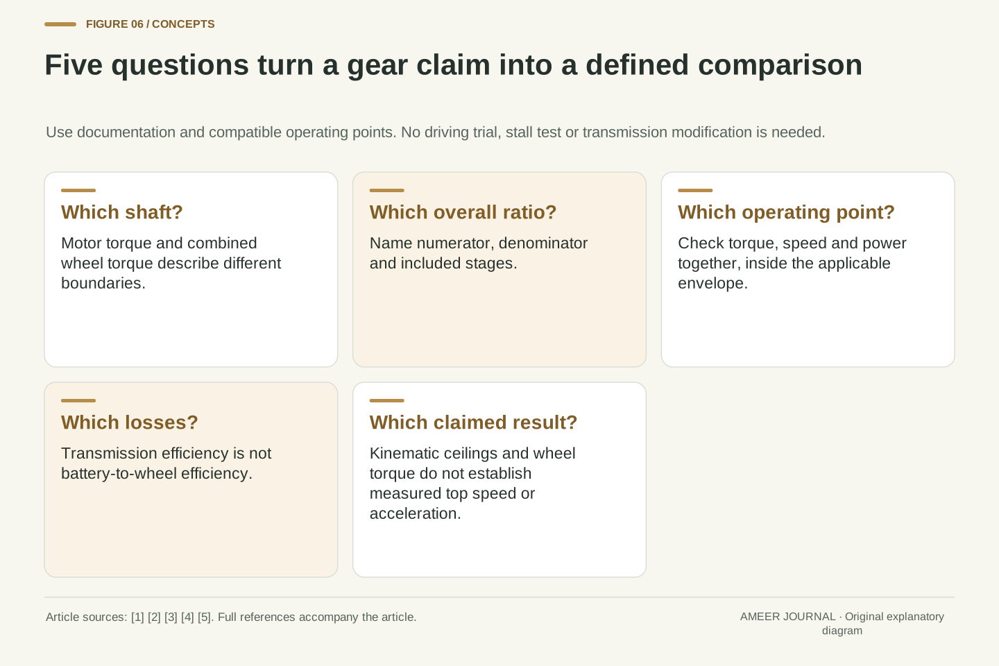
Start a specification comparison by locating the torque number: motor shaft, intermediate shaft or combined wheel output. Then identify the overall ratio and the wheel-speed conversion. Next ask where the claimed point lies on the motor's operating envelope and what efficiency boundary is being used. The DOE component map, gear relationships and motor-model descriptions support these as separate questions. [1][2][3] A larger torque number after reduction may simply describe a different shaft turning more slowly.
The imaginary example provides a reusable check. Nine motor turns produce one wheel turn; 200 newton-metres becomes an assumed 1,710 at the combined output after losses; 100.53 kW becomes 95.50 kW rather than increasing. At a different road speed or motor limit, the same ratio can lead to a different available torque. Reading all of those quantities together gives single-speed its proper meaning: one fixed speed relationship across a changing operating range. It answers the mechanical question while leaving real acceleration, efficiency and maximum speed to evidence about the actual vehicle and conditions.
For any claimed advantage, identify the input/output shafts, ratio convention, motor operating point, rolling conversion and energy boundary. Check whether maximum torque and maximum power are being compared at compatible speeds. If a ratio changes, hold the stated comparison variables fixed explicitly: equal motor speed, equal road speed and equal input power are different experiments. The cited mechanical and motor references provide the relationships needed to keep those comparisons consistent. [2][3][4]
The baseline's G = 9, ηg = 0.95, Tm = 200 N·m and nm = 4,800 rpm yield a coherent set of shaft quantities. The six-versus-nine comparison then changes the operating point at fixed road speed, while the constant-power example changes how available motor torque depends on speed. None creates power through gearing. Those three calculations explain the useful design trade-off without converting an invented envelope into a product rating. A defensible single-speed claim connects a fixed kinematic ratio to a specified, variable motor operating region and reports the wheel-side result at the correct boundary.
Sources & further reading
Explore the references behind this guide. External pages may change after our review.
- Alternative Fuels Data Center: How Do All-Electric Cars Work?U.S. Department of Energy — Alternative Fuels Data Center · Accessed 6 Nov 2026
- Couple Rotational Motion with Gears - MATLAB & SimulinkMathWorks · Accessed 6 Nov 2026
- Motor & Drive - Generic motor and drive with closed-loop torque control - MATLABMathWorks · Accessed 6 Nov 2026
- Choosing a Motor and Gearing Combination - Northwestern Mechatronics WikiNorthwestern University — Mechatronics · Accessed 6 Nov 2026
- Technical Feature: The Porsche Taycan - Porsche Newsroom AUSPorsche Newsroom · Accessed 6 Nov 2026
Article updated 6 Nov 2026.
Found something we should revisit?
Good explanations get better with thoughtful feedback.