What you’ll take away
- Estimated kilometres combine an energy budget with a reference or assumption about consumption; they do not count distance already travelled.
- A changed forecast can alter remaining range without consuming the energy it predicts will be needed later.
- Match battery-side or wall-side energy boundaries before dividing an energy budget by consumption per distance.
- A combined consumption average uses total energy divided by total distance, and the chosen history window still matters.
- Compare a forecast with the same journey, time and boundary, while following the particular vehicle’s warnings and guidance.
A falling estimate does not count kilometres already travelled
Suppose an electric car shows 200 kilometres of remaining range, then shows 140 after a 10-kilometre journey. It is tempting to say that 50 kilometres of battery capacity have disappeared. But kilometres are not a quantity of stored energy. A remaining-distance estimate connects energy available now with an assumption about energy use ahead. Changing either part can change the answer. Ford’s range-display documentation explicitly identifies available battery energy and driving consumption as separate influences on its estimate. [3]
This article follows that distinction through original paper calculations. All energy amounts, consumption rates, distances and forecast errors below are invented; no vehicle was driven, charged or measured. When we name an energy budget, it means energy available for the stated illustrative calculation, not a recommendation to use every last part of a battery. The task is to read the estimate’s meaning, not to prove a car’s endurance by driving it to depletion. We will keep three things separate: energy already used, the recent history being summarized and the future journey being predicted.
Remaining range is a derived distance, not an odometer or a direct capacity measurement. A simple explanatory model divides an available travel-energy budget E by assumed future energy consumption per distance q. Both the energy estimate and the forecast basis can matter. Ford’s retrieved range-display page describes dependence on driving energy use and available high-voltage-battery energy, while Tesla’s manual distinguishes rated and consumption-based displays. Those sources do not specify one universal estimator for all vehicles. [2][3]
The original models below declare E in kWh and q in kWh/km at the battery-withdrawal boundary. They omit charging during the stated journey and keep any separately specified stationary use outside the driving-rate term. Inputs are stipulated, not measured vehicle data, a battery-capacity test or a production forecasting algorithm. A range change will be attributed only within the stated sequence of assumptions. In particular, a changed forecast must not be silently treated as energy already consumed, and a convenient distance quotient must not be substituted for the applicable vehicle warnings or trip-planning guidance.
A rated reference, recent history and a route forecast answer different questions
First identify which number you are reading. The retrieved Model 3 manual for the Ireland locale describes the main distance display using EPA-rated consumption. It separately describes projected range based on remaining energy and average consumption, and a trip view that compares actual usage with a navigation projection. These are different reference choices within that documented system. They need not give identical answers because one asks about a fixed reference, another about recent usage and another about the planned trip. [2]
A number on a vehicle’s sales label has a different purpose again. EPA explains that laboratory driving cycles, adjustments and combined results produce the labelled range. That creates a defined comparison rather than a promise to match every later journey. [1] Polestar’s 2023 US manual also describes different range-display choices and separate short/long estimates tied to different consumption scenarios. Those scenario endpoints are not stated as statistical confidence limits. [4] The useful first step is therefore to read the display’s definition, rather than assume that every number called “range” uses yesterday’s driving in the same way.
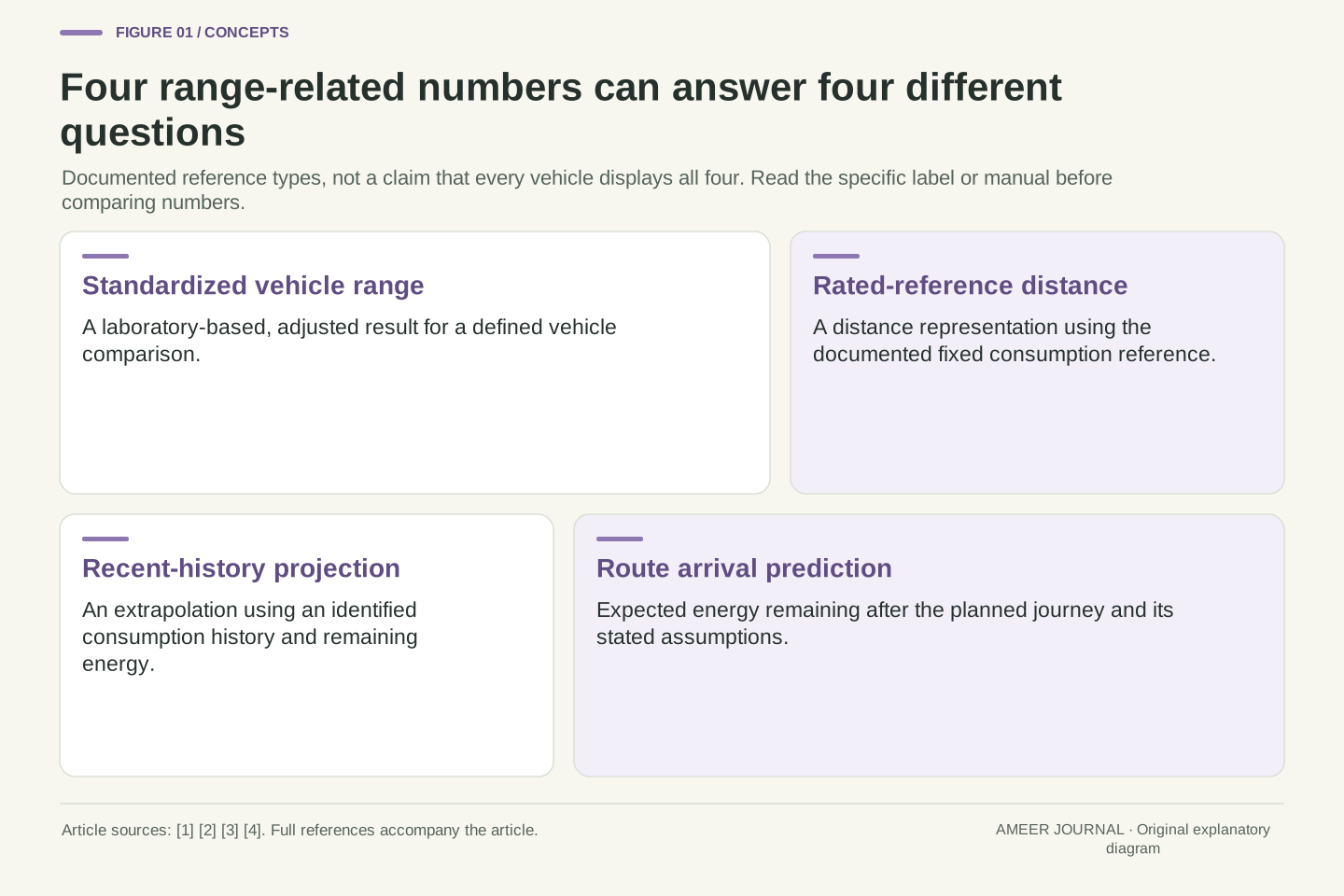
Distinguish a standardized vehicle-range result, a distance representation using a fixed reference consumption, a recent-consumption extrapolation and a route-conditioned energy prediction. EPA’s documented range procedure uses laboratory cycles and adjustments to generate a combined label result. It is not a live estimate of one driver’s remaining trip. The exact Model 3 regional manual supplies a separate example of rated consumption, historical-average projected range and comparison with a navigation projection. [1][2]
These categories describe reference choices, not an asserted implementation shared across brands. The same manual’s mention of an EPA-based reference does not establish that its internal conversion simply divides battery energy by the wall-side consumption printed on an EPA label. Measurement boundaries still need to match. Polestar’s exact 2023 US documentation describes scenario-dependent short and long values and display choices; it does not label those scenario values as probabilistic bounds. Name the displayed quantity and its reference before judging whether two estimates disagree. [1][2][4]
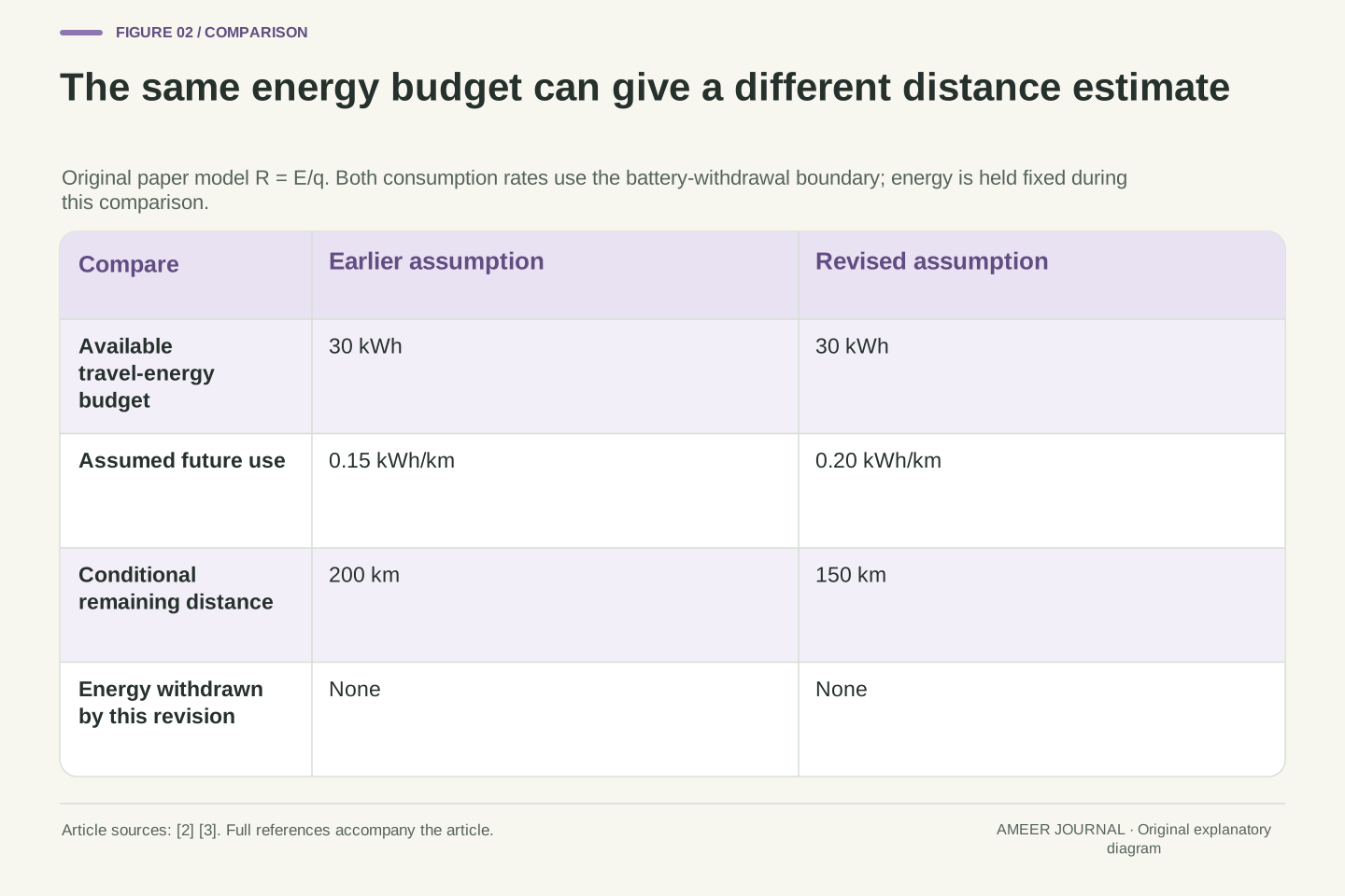
The same 30 kWh can imply 200 kilometres or 150 kilometres
Take an illustrative energy budget of 30 kWh. If the assumed future use is 0.15 kWh for each kilometre, divide 30 by 0.15: the result is 200 kilometres. The same rate can be written as 15 kWh per 100 kilometres. Now keep the energy budget exactly the same but change the future-use assumption to 0.20 kWh per kilometre, or 20 kWh per 100 kilometres. The answer becomes 150 kilometres. The 50-kilometre difference comes entirely from the changed assumption in this model.
Nothing in that second calculation says 50 kilometres have been driven or that a corresponding block of battery energy has vanished. The estimate is answering a new conditional question: how far the unchanged budget would cover at the newly assumed rate. Tesla’s documented projected-range description connects remaining energy with average consumption, and Ford describes variation with energy use and conditions. [2][3] Those real descriptions motivate the relationship, but our two rates and 30 kWh budget are deliberately fictional. If a real vehicle also revises its available-energy estimate, that would introduce a second changing quantity that this particular comparison holds fixed.
For q>0, the explanatory quotient R=E/q has units kWh/(kWh/km)=km. At E=30 kWh, q0=0.15 kWh/km gives R0=200 km; q1=0.20 kWh/km gives R1=150 km. Holding E fixed produces ΔR=−50 km without energy withdrawal. The sensitivity is inverse rather than additive: increasing q by one third reduces R by one quarter. A percentage increase in consumption is therefore not the same percentage decrease in distance.
The model is consistent with the documented role of remaining energy and average consumption, but no manufacturer is claimed to implement exactly this quotient without other terms. [2][3] More generally, for positive E and q, R1/R0=(E1/E0)(q0/q1). Different combinations of energy and rate changes can yield the same range ratio. A single displayed distance change cannot uniquely recover both causes. Here E1/E0=1 by construction; a real available-energy revision, rounding policy or additional route term would need its own evidence rather than being inferred from the fictional arithmetic.
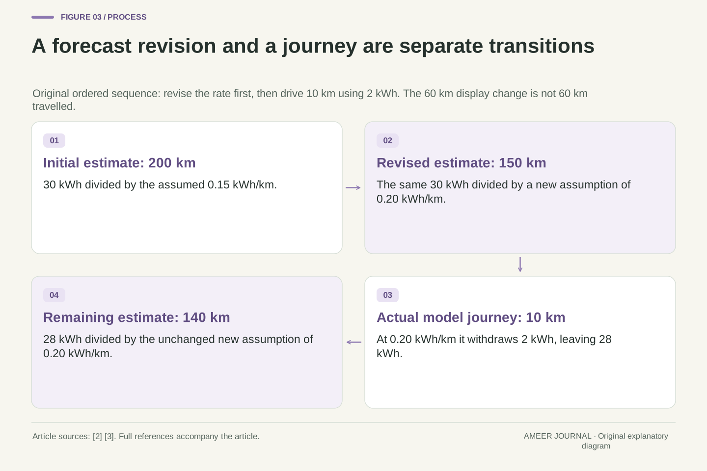
A ten-kilometre journey can accompany a sixty-kilometre display drop
Continue the same invented sequence in a stated order. First, the future-use assumption changes from 0.15 to 0.20 kWh per kilometre while the 30 kWh budget stays unchanged. The display moves from 200 to 150 kilometres. Then the car in our paper story travels 10 kilometres and actually uses 0.20 kWh per kilometre. That journey withdraws 2 kWh, leaving 28 kWh. If the new forecast rate stays at 0.20, the remaining-distance estimate becomes 140 kilometres.
The full display decrease is 60 kilometres, but the travelled distance is 10 kilometres and the energy used is 2 kWh. In this explicitly ordered example, 50 kilometres of the estimate change came before the journey from the forecast revision; the next 10 came from travel at the new assumed rate. No extra “missing 50 kilometres” has to be converted into an unexplained energy loss. The retrieved Model 3 documentation specifically warns that displayed range may decrease faster than actual distance travelled. [2] Its real display behaviour has its own reference; our sequence explains the distinction without claiming to reproduce its software.
Even an unchanged reference can produce a faster drop. In a separate version, keep the original 0.15 reference while actually using 2 kWh over the same 10 kilometres. The estimate moves from 200 to about 186.7 kilometres: a 13.3-kilometre decrease. The reference converts each kWh into more estimated distance than this particular trip achieved. No forecast revision is needed for that difference.
Separate two transitions. Forecast update: (E,q)=(30,0.15) becomes (30,0.20), so R changes from 200 to 150 km. Travel transition: d=10 km at actual battery-side use q_actual=0.20 kWh/km withdraws ΔE=q_actual d=2 kWh. With q held at 0.20 afterward, the state becomes (28,0.20) and R=140 km. The total estimate change is −60 km; the actual path length is 10 km.
The 50-plus-10 decomposition is justified by that stated sequence, not a unique attribution recoverable from arbitrary before/after readings. If energy and forecast terms change together, different intermediate counterfactuals can partition the same total difference differently. What remains certain in this example is the declared energy withdrawal and the endpoints. Tesla’s manual supports the observation that displayed-distance reduction need not match odometer distance; it does not supply these values or this algorithm. [2] Keeping the order explicit prevents a forecast correction from being counted again as an additional physical energy withdrawal.
A separate fixed-reference case needs no revision at all. Hold q_reference=0.15 kWh/km while q_actual=0.20 over d=10 km. E falls from 30 to 28 kWh, so the display quotient falls from 200 to 560/3 km, about 186.7. Generally, with a constant positive reference and only the stipulated trip withdrawal, R_before−R_after=q_actual d/q_reference. Here the displayed decrement is 40/3 km, or 4/3 times the actual distance. This is the difference between reference-normalized distance and achieved travel, not an additional energy-loss term. The underlying withdrawal remains 2 kWh; counting the excess displayed decrement as another withdrawal would count the same energy through two incompatible conversions.
The energy numerator and the consumption denominator must use the same boundary
An electricity bill records energy supplied during charging. A driving calculation may instead count energy withdrawn from the battery. They are related, but charging is not perfectly efficient. EPA explicitly states that its MPGe values include charging losses, placing the measurement at the wall rather than only at the vehicle’s battery. [1] A familiar-looking consumption figure can therefore be the wrong denominator for a battery-side energy budget, even when both are written in kWh per distance.
Consider a separate invented example: restoring 18 kWh of battery energy requires 20 kWh from the wall, and that 18 kWh supports a 100-kilometre trip. The battery-side trip rate is 0.18 kWh per kilometre; the corresponding wall-input rate is 0.20. If a later illustrative battery budget is 27 kWh, using the battery-side rate gives 150 kilometres. Dividing by the wall-side rate gives 135 kilometres, answering a mismatched calculation. The point is not that one rate is false. Each can be correct for its own boundary. The error is combining the energy available inside one boundary with a rate measured outside it.
Define the numerator and denominator at the same energy-accounting boundary. EPA’s MPGe description includes EVSE and on-board conversion losses under its stated charging basis. Thus a wall-side consumption figure cannot automatically be used with a battery-withdrawal budget. [1] This is separate from whether a given vehicle’s range estimator applies a calibrated rated reference internally; the public label alone does not reveal that implementation.
In the separate original cycle, wall input is 20 kWh, restored battery energy is 18 kWh and subsequent trip withdrawal is 18 kWh over 100 km. The stipulated charging-energy ratio is 18/20=0.9. Then q_battery=18/100=0.18 kWh/km and q_wall=20/100=0.20 kWh/km. With a later E_battery=27 kWh, E_battery/q_battery=150 km, whereas E_battery/q_wall=135 km mixes boundaries. No real charging efficiency is being estimated. Other charging-session loads or changes in stored energy would need to be explicitly included before interpreting a real recharge-to-trip comparison.
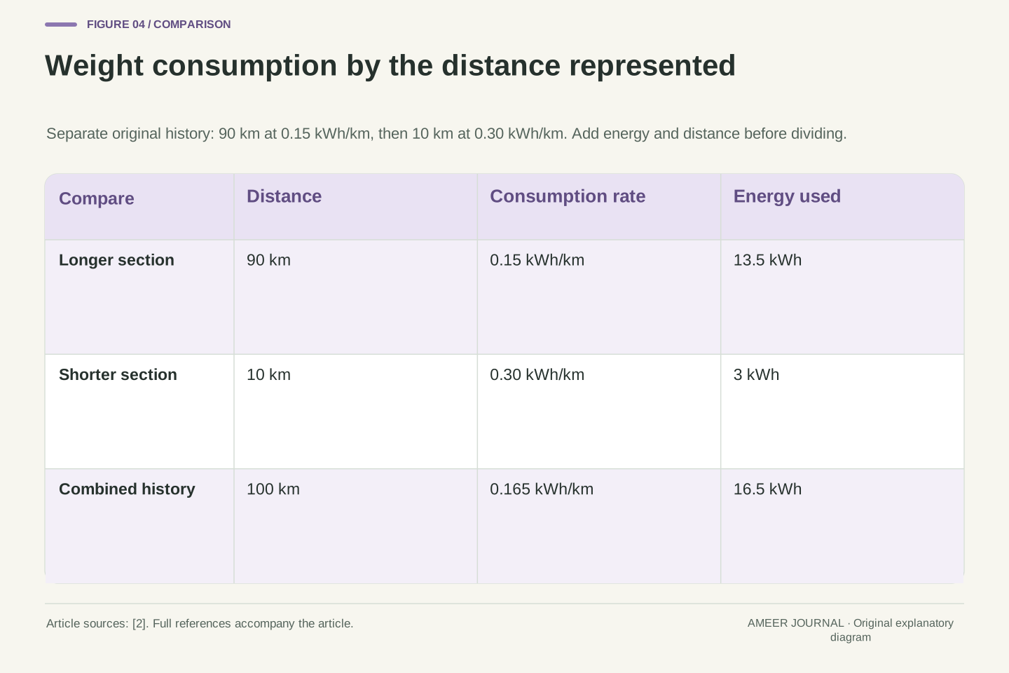
Add the energy and distance before averaging consumption
A history average needs another careful denominator. Imagine a recent record containing 90 kilometres at 0.15 kWh per kilometre, followed by 10 kilometres at 0.30. The first part uses 13.5 kWh; the second uses 3 kWh. Together they use 16.5 kWh over 100 kilometres, so the distance-based average is 0.165 kWh per kilometre. Each kilometre contributes to the total; the short section does not receive the same weight as the long one merely because it occupies one row in a table.
Simply averaging the two rates would give 0.225 kWh per kilometre. That would be correct for equal distances at those rates, but the stated distances are not equal. With a separate current budget of 30 kWh, extrapolating the actual combined average gives about 181.8 kilometres. Using the unweighted rate would give about 133.3 kilometres. Neither result is a promise about future driving: this comparison isolates an arithmetic error before we even ask whether the history represents the next trip. Tesla’s manual describes projected range using average energy per distance; the correct averaging basis is therefore part of understanding such a quantity. [2]
For distance-based consumption q_i over segment distance d_i, total energy is Σ(q_i d_i) and the combined rate is q_bar=Σ(q_i d_i)/Σd_i, provided the accounting boundaries agree. The original segments give 0.15×90=13.5 kWh and 0.30×10=3 kWh. Thus q_bar=16.5/100=0.165 kWh/km, with distance weights 0.9 and 0.1. This is a defined aggregate, not a claim about hidden vehicle filtering.
The unweighted expression (0.15+0.30)/2=0.225 kWh/km assumes equal distance weights. With E=30 kWh, the two extrapolations are 30/0.165=2000/11 km, about 181.8, and 30/0.225=400/3 km, about 133.3. In reciprocal units the correct aggregate is 100/16.5=200/33 km/kWh, about 6.061; one cannot generally average reciprocals with the same weights and expect the reciprocal result. The manual’s average-consumption description supports the relevance of the unit, while the weighting and arithmetic here are original definitions. [2]
A correct history average can still be a poor description of what comes next
Return to that 100-kilometre history. Looking only at its last 10 kilometres gives 0.30 kWh per kilometre, while the complete record gives 0.165. Both are correctly calculated averages of the periods they describe. With the same illustrative 30 kWh budget, they imply 100 kilometres and about 181.8 kilometres respectively. The difference is not proof that either historical record is inaccurate. It shows that the chosen window is part of the estimate.
A shorter window responds strongly to the recent high-use section. A longer window retains more of the earlier lower-use section. Tesla’s retrieved manual explicitly describes selectable history distances and notes that a longer distance stabilizes projected range. [2] Stability does not establish that the next journey will resemble the older record. A past urban journey and a future motorway journey may require different assumptions. Polestar’s scenario-based short and long figures likewise tie their meaning to stated driving and climate conditions. [4] Before interpreting a change as a fault, ask whether the reference period or future scenario changed as well.
The windowed averages describe different datasets: q_last10=0.30 kWh/km, while q_last100=0.165 kWh/km. At E=30 kWh, their direct extrapolations are 100 km and 2000/11 km. This original example isolates window selection without adding smoothing coefficients, route learning or a claimed manufacturer algorithm. No forecast can be evaluated solely by whether its historical average was arithmetically correct.
Tesla’s manual states that a longer selected history stabilizes projected range and captures driving behaviour, environment and routes. [2] The statistical interpretation still depends on future relevance: retaining older observations reduces the influence of one short segment but can delay adaptation to a sustained change. That is a property of the stated window comparison, not measured forecast performance. Polestar’s documented high/low-consumption scenarios illustrate another conditional basis; their endpoints describe assumptions rather than probabilities. [4] A stable estimate, a responsive estimate and an accurate prediction for a particular upcoming route are distinct qualities.
Zero distance travelled does not require zero energy use
The opposite mistake is to assume every change while parked is only a revised forecast. A stationary vehicle can use energy without travelling any distance. The Ford page identifies battery energy used to support the accessory battery while unplugged, and Tesla’s Energy app documentation includes a parked-energy account. [2][3] Actual consumption and a changed expectation are different explanations, and both are possible categories of change.
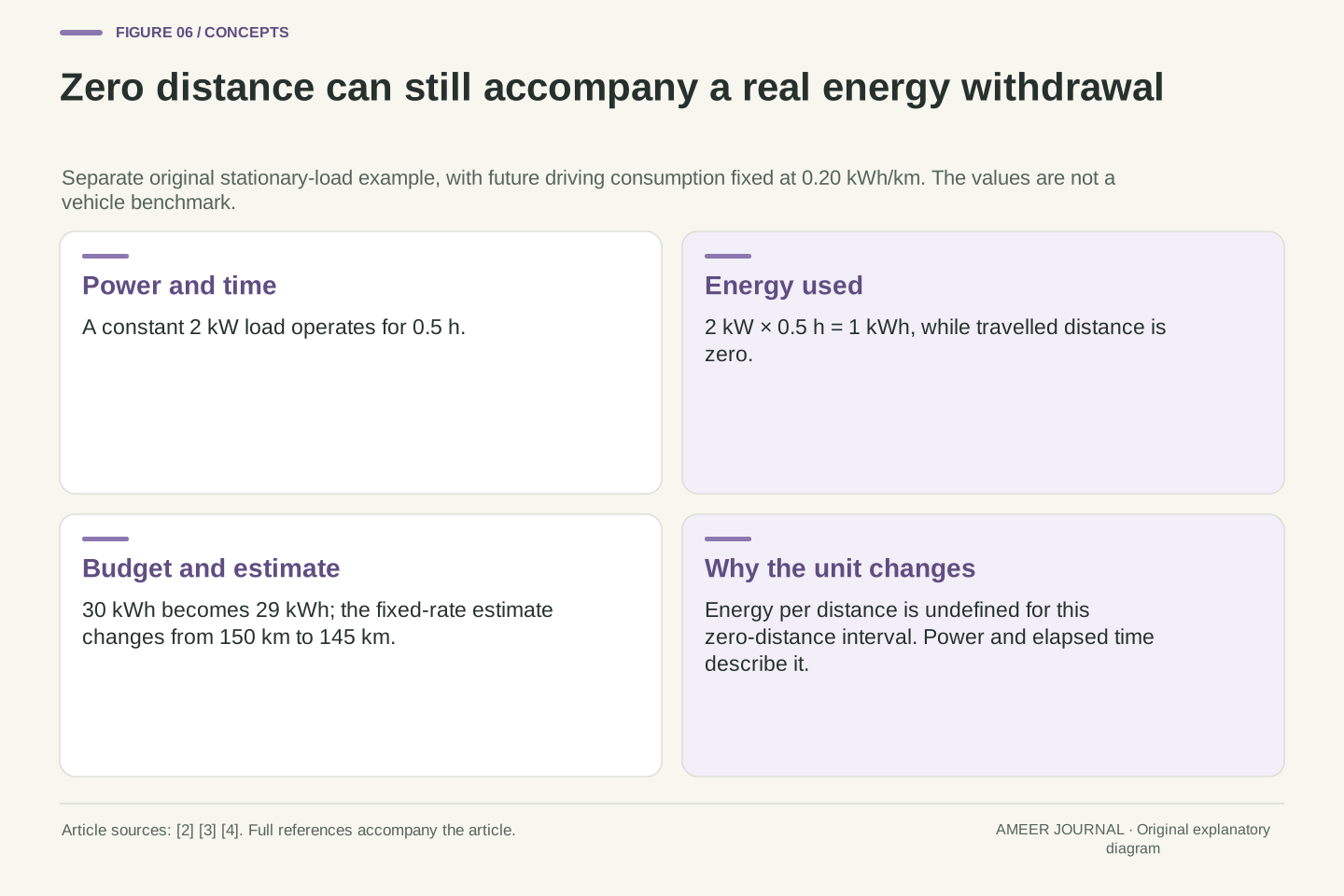
For a separate paper example, let a constant 2 kW battery load operate for half an hour. It uses 1 kWh even though distance travelled is zero. An illustrative 30 kWh budget becomes 29 kWh. With the future driving rate held at 0.20 kWh per kilometre, the estimate falls from 150 to 145 kilometres. Here the five-kilometre drop corresponds to an actual energy withdrawal under the fixed conversion. A distance-based rate for the stationary interval would involve division by zero, so it is not meaningful. Polestar’s cited manual uses power units while stationary and energy-per-distance units while moving, making that distinction explicit. [4]
For stationary consumption, energy follows the time integral of power rather than a positive distance denominator. In the original constant-load case, E_used=(2 kW)(0.5 h)=1 kWh. Starting from a 30 kWh illustrative budget gives 29 kWh after the interval. Holding q_future=0.20 kWh/km fixed changes R from 150 to 145 km. This is an energy-use transition, unlike the earlier fixed-energy forecast transition.
The interval’s distance is zero, so E_used/d is undefined; reporting a finite kWh/km value for that interval would invent a denominator. Polestar’s specific manual describes displaying kW when stationary and kWh/100 km when moving. Ford documents an unplugged accessory-battery support draw, and Tesla documents a parked-energy view. [2][3][4] These establish that parked energy use is a real accounting category, not that the fictional 2 kW load is typical or that a particular vehicle must lose five kilometres. No feature-disabling or safety-climate recommendation follows from the example.
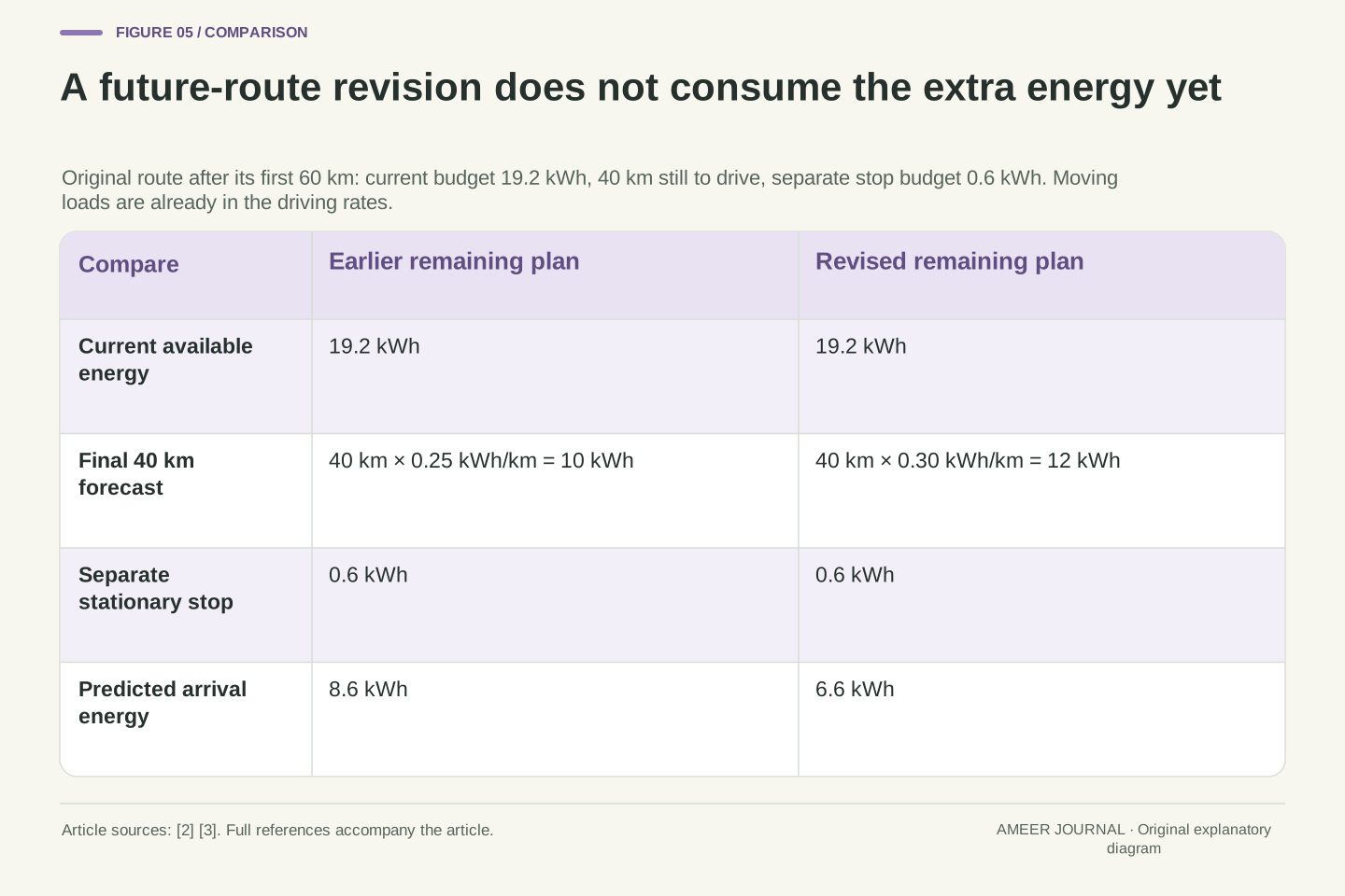
A route forecast can update the future without rewriting energy already used
A route budget can work forward segment by segment. Start a new invented journey with 30 kWh. Assume 60 kilometres at 0.18 kWh per kilometre, then 40 kilometres at 0.25, plus a separate stationary stop using 0.6 kWh. The driving rates already include all moving-vehicle loads in this model, so the stop is not counted twice. The forecast uses 10.8+10+0.6=21.4 kWh and leaves 8.6 kWh on arrival. Tesla’s trip view provides a real example of comparing actual usage with a destination-based projection, without supplying this simplified model. [2]
Suppose the first 60 kilometres use exactly the expected 10.8 kWh. The current budget is 19.2 kWh, and the unchanged remaining plan still leaves 8.6 kWh at arrival. Now revise only the final 40-kilometre forecast to 0.30 kWh per kilometre. Its expected energy rises from 10 to 12 kWh, reducing predicted arrival energy to 6.6 kWh. The current 19.2 kWh has not changed at the instant of that revision. Two extra kWh are expected to be used later; they have not already been consumed.
For the original segmented route, define E_arrival=E_now−Σ(q_i d_i)−E_stop. With E_now=30 kWh, q1=0.18 kWh/km over 60 km, q2=0.25 kWh/km over 40 km and E_stop=0.6 kWh, forecast withdrawal is 21.4 kWh and arrival energy is 8.6 kWh. Driving q_i already includes moving auxiliary use; the separate stop is additional stationary consumption. Tesla’s documented trip projection motivates the distinction between current energy and predicted destination energy, not these assumed coefficients. [2]
After segment 1 matches prediction, current E is 19.2 kWh. Remaining forecast 10+0.6 kWh still gives 8.6 kWh on arrival. Revising only q2 to 0.30 kWh/km changes the remaining forecast to 12+0.6 kWh and arrival prediction to 6.6 kWh. The revision increases forecast future use by 2 kWh while leaving present E unchanged. This is not a revised physical history. The model keeps the same route length, stop and boundary so that the effect of one future assumption is identifiable; real navigation forecasts can update several inputs together.
Compare a prediction with the same journey and energy boundary
To evaluate a forecast, preserve what it predicted before comparing it with what happened. In a separate completion of the original route, suppose the prediction was 21.4 kWh but actual withdrawal was 22.5 kWh. The energy-use error is 1.1 kWh. Starting from 30 kWh with no recharge would leave 7.5 kWh rather than the predicted 8.6. These two errors agree because they describe the same journey and accounting boundary, with opposite signs for energy used and energy left.
A real comparison needs the same discipline. A prediction made before departure and one revised halfway through are different forecasts. Energy figures that already depend on the same internal estimate do not become independent battery measurements merely because they appear on different screens. Ford’s documentation identifies both consumption and available-energy effects, so a changed range number alone cannot diagnose which changed. [3] Read the vehicle’s own warnings and guidance, and review records only when safely parked. The useful record names the starting point, route, display definition and later result rather than treating one surprising number as a battery-health test.
Define the original forecast-use residual as actual minus predicted withdrawal: r_E=22.5−21.4=+1.1 kWh. With the same stipulated 30 kWh initial budget and no charging, actual arrival energy is 7.5 kWh versus predicted 8.6 kWh, so the arrival residual is −1.1 kWh. This consistency follows from matched boundaries and endpoints. It would not hold unchanged if a later reforecast, extra charging, a different route or another energy boundary were substituted.
Forecast validation also needs a suitable observation. Two displays derived from the same underlying energy estimate are not automatically independent measurements of capacity. The documented dependence on available energy and consumption creates an identification problem: range alone does not isolate degradation, temperature effects or a changed forecast. [3] A useful comparison therefore labels prediction time, assumptions, route, observed interval and measurement provenance. The fictional residual is an accounting check, not evidence of predictive accuracy for Tesla, Ford, Polestar or any real vehicle.
Read the estimate as a conditional statement
A useful remaining-range statement can be read as a sentence: with this energy budget, under this reference or future-use assumption, the estimated distance is this much. That wording makes the missing information easier to spot. Is the number based on a rated reference, a recent distance window or a planned route? Does consumption count battery withdrawal or charging input? Does a comparison cover the same period? The official sources use different definitions, and those definitions matter more than the familiar unit “kilometres”. [1][2][3][4]
The paper examples show several distinct causes of movement in the number. A forecast rate can change with no energy withdrawal. A short journey can follow that revision. Parked equipment can use energy without distance. A correctly averaged history may differ from the next route. None of those explanations makes every surprising estimate harmless or identifies a particular battery fault. They show why the distance display needs context, while the vehicle’s warnings and documented operating guidance still apply. Keep the forecast, the energy account and the actual journey separate, and the number becomes much easier to interpret.
Treat remaining range as a conditional derived quantity whose numerator, denominator and reference period must be identified. A standardized label, rated-distance display, historical extrapolation and route-arrival estimate provide different information. Their legitimate differences are not resolved by choosing the largest number or assuming a common algorithm. The cited documents establish those distinctions and the role of energy use, available energy, history and operating conditions. [1][2][3][4]
The original calculations add an interpretable accounting structure: R=E/q for a stated common boundary, explicit transition order, distance-weighted history, a defined observation window, stationary energy integration and separate future route terms. Comparing a forecast with a matched later result then exposes the residual without relabelling it as capacity loss. These relationships explain why estimated kilometres need not decrease one-for-one with travelled kilometres. They remain a reading framework, not a depletion test, a manufacturer algorithm reconstruction or a substitute for the particular vehicle’s warnings and instructions.
Sources & further reading
Explore the references behind this guide. External pages may change after our review.
- Fuel Economy and EV Range Testing | US EPAU.S. Environmental Protection Agency · Accessed 7 Nov 2026
- Getting Maximum RangeTesla · Accessed 7 Nov 2026
- Instrument Cluster — Vehicle Range DisplayFord Motor Company · Accessed 7 Nov 2026
- Range assistantPolestar · Accessed 7 Nov 2026
Article updated 7 Nov 2026.
Found something we should revisit?
Good explanations get better with thoughtful feedback.