What you’ll take away
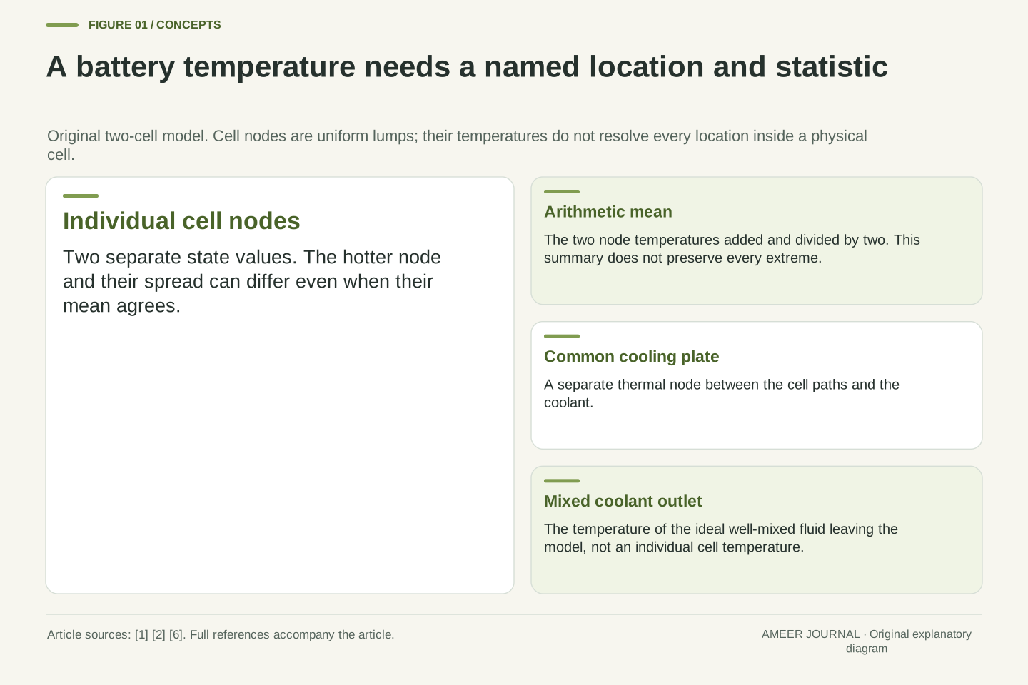
- A temperature needs its location and aggregation rule: coolant, plate, individual cell and average are different quantities.
- Equal average cell temperatures can coexist with different maxima and temperature spreads.
- Even matching individual temperatures need not identify whether generation or thermal resistance caused them.
- Coolant heat flow depends on flow rate and temperature change together; a smaller rise does not necessarily mean less heat removal.
- Thermal capacity affects the response to a change, while steady temperatures depend on heat generation, paths and boundary conditions.
A temperature needs a location before it can tell a story
A report says an electric vehicle’s battery coolant leaves a cooling plate at 18°C. Does that mean every cell is near 18°C? The reading describes the coolant at that location. It does not automatically describe the cells, the plate, the hottest spot or the average across the pack. NLR’s battery research treats temperature and temperature uniformity as separate matters, and examines cells, modules and complete systems. [1]
There is a useful reason to keep those labels separate. Heat must travel from where it is generated to somewhere that can receive it. Along that route, different parts can have different temperatures. An indirect cooling arrangement described by Southwest Research Institute carries heat from cells through a plate or similar structure into flowing coolant. The fluid then carries the energy onward to a heat exchanger. [2]
We will build an original, invented two-cell model to find out how much a coolant reading actually reveals. Each cell has one uniform temperature in the model, so it cannot resolve hotter regions inside a real cell. All temperatures, heat rates and material values below are stipulated teaching numbers, not measurements, operating targets or safety limits. The interesting result is that the same average can hide different extremes.
A reported battery temperature is incomplete without its measurement or model location and aggregation rule. A coolant outlet temperature, a cold-plate temperature, a cell-node temperature and a pack statistic are different observables. NLR identifies both temperature and temperature uniformity as relevant to battery assessment; its public 2024 research abstract also distinguishes heat sources and cooling arrangements at different assembly levels. [1][6]
The question here is an inverse problem: which internal states are consistent with a small set of reported temperatures? Rather than assume that the outlet represents every cell, we will construct several states with identical outlet and arithmetic-mean values. A counterexample is sufficient to show that those two values alone do not uniquely determine the maximum cell-node temperature.
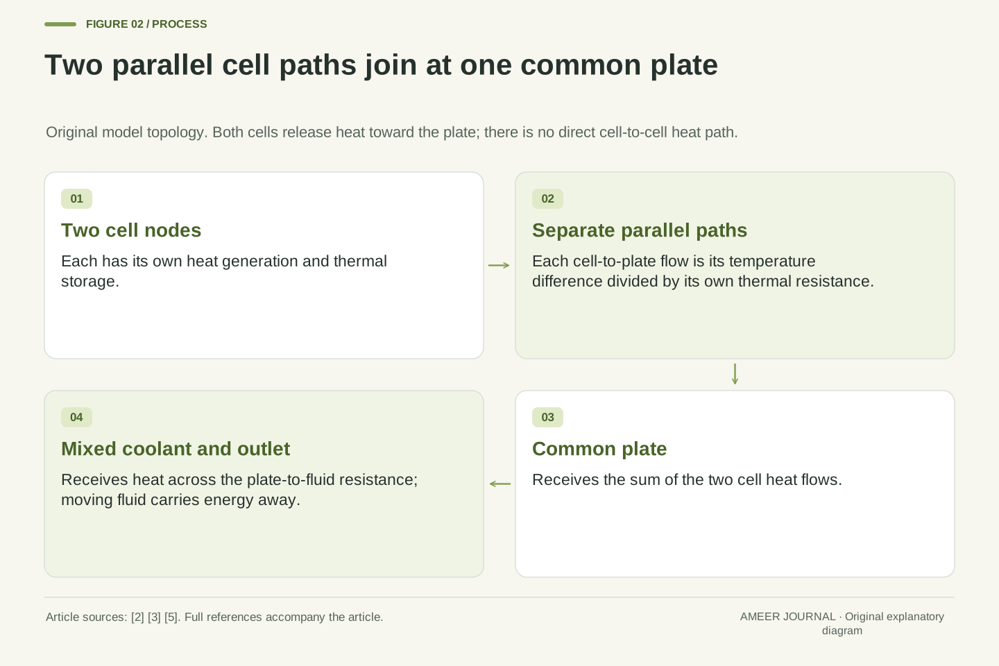
The original model contains two internally uniform cell lumps, separate paths to one common plate and an ideal well-mixed coolant node whose temperature equals its outlet temperature. Parameters are constant, other heat paths and sources are omitted, and the inlet is prescribed. Every numerical value is invented. This restricted network tests inference from temperatures; it does not reproduce an EV, resolve intra-cell gradients or specify an acceptable operating temperature.
Heat generation and temperature rise are different quantities
A watt measures an energy-transfer rate: one joule each second. A temperature tells us the thermal state of the part we are describing. A cell can keep generating heat while its temperature stays steady, provided energy leaves at the same rate. If more enters its thermal store than leaves, that store grows. The thermal-mass relation in MathWorks documentation connects the net heat rate to the rate of temperature change. [4]
Give each invented cell a heat capacity of 240 joules per kelvin. This means adding 240 joules to its thermal store raises its model temperature by one degree, with that capacity held constant. If it generates 6 watts while 4 watts leave, the net addition is 2 watts. Dividing 2 by 240 gives an instantaneous rise rate of one hundred-and-twentieth of a degree per second.
That rate is equivalent to half a degree per minute at that instant. It does not promise a half-degree rise over the next minute: as the cell warms, its heat loss may change. Conversely, an unchanged temperature does not mean nothing is happening. It may mean a continuous stream of energy is being generated and removed at matching rates. That is the condition used in our first comparison.
For a constant-capacity cell node, write C dT/dt = P − Q, where C is heat capacity in J/K, P is internal heat generation in W and Q is heat transferred out in W. The thermal mass documentation gives the corresponding constant-mass relation between net heat flow, mass, specific heat and temperature derivative. Here C is a thermal storage parameter, not electrical capacity in ampere-hours. [4]
With C = 240 J/K, P = 6 W and Q = 4 W, the instantaneous derivative is 2/240 = 1/120 K/s, equivalently 0.5 K/min. The conversion changes the time unit, not the assumption about how long that derivative persists. Integrating a fixed rate over a finite interval would require the net heat input to remain fixed over that interval.
Steady temperature requires P = Q for this node, not P = 0. The distinction matters when interpreting a flat trace: thermal energy can pass through continuously without accumulating. Temperature differences have the same numerical size in kelvins and degrees Celsius, but absolute Celsius readings should not be treated as ratios. None of the comparisons below interprets 32°C as twice the thermal state of 16°C.
The heat path needs a temperature difference
Our model gives each cell its own path to the common plate. A thermal resistance describes how much temperature difference that path needs to carry a given heat rate. In the constant-resistance relation, temperature difference equals heat rate multiplied by resistance. The units are kelvins per watt. This is a heat-flow model, not an electrical resistance or a guide to the construction of a battery. [3]
Suppose the plate is at 20°C and a cell sends 6 watts through a path of 2 kelvins per watt. The required difference is 6 × 2 = 12 kelvins, so the cell node is at 32°C. A second cell sending only 2 watts through the same resistance needs a 4-kelvin difference and sits at 24°C. Both transfer heat toward the same cooler plate.
The path matters as much as the destination. A larger resistance needs a larger temperature difference for the same heat flow. SwRI’s account explains why the conductivity of an indirect cooling path can constrain heat removal. [2] The resistance here bundles the path into one number. It leaves us able to ask a clear question: did a cell become hotter because it generated more heat, or because its route to the plate transferred heat less readily?
Use Q_i = (T_i − T_p)/R_i for each cell-to-plate branch, with positive Q_i directed toward the plate. This is the constant thermal-resistance relation RQ = ΔT documented by MathWorks. R_i has units K/W. The two branches are parallel connections to a shared node; heat from cell A does not first pass through cell B. [3]
At steady state, Q_i = P_i, giving T_i = T_p + P_i R_i. For T_p = 20°C, P_A = 6 W and R_A = 2 K/W, T_A = 32°C. With P_B = 2 W and R_B = 2 K/W, T_B = 24°C. The temperature offsets are 12 K and 4 K, respectively. Their arithmetic follows from the stipulated branch parameters, not from a universal cell-to-coolant offset.
An effective resistance can summarize a path without identifying every material or interface inside it. SwRI discusses the importance of the conductivity of the cooling pathway; the abstract resistance model deliberately suppresses that geometry. [2][3] If the plate were hotter than a cell, the sign of this same equation would reverse. The equation describes a directional energy balance, not an assertion that every thermal-management state must be cooling.
Three different interiors can share the same average
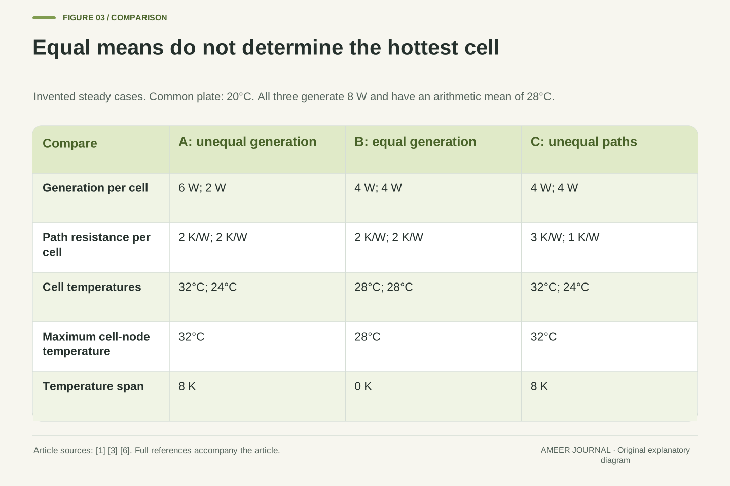
Call the 6-watt and 2-watt arrangement case A. Its cell temperatures are 32°C and 24°C, so the simple average is 28°C. The hottest cell node is 32°C and the difference between the two is 8 degrees. Now make case B: each cell generates 4 watts and each path still has a resistance of 2 kelvins per watt. Both cells settle at 28°C when the plate is at 20°C.
Cases A and B generate the same total heat: 8 watts. They have the same average cell temperature, but different maxima and different temperature spreads. Case B’s maximum is 28°C and its spread is zero. A report containing only the average would make these different interiors look identical. Temperature uniformity therefore adds information that a mean by itself cannot carry. [1]
There is a third possibility. In case C, keep generation equal at 4 watts per cell, but give the paths resistances of 3 and 1 kelvin per watt. The temperature differences above the plate become 12 and 4 degrees. The cell readings are again 32°C and 24°C, exactly like case A. Equal readings do not even establish whether unequal generation or unequal paths produced them.
At the common plate temperature of 20°C, compare three steady states. A has generation (6, 2) W and resistances (2, 2) K/W, producing temperatures (32, 24)°C. B has generation (4, 4) W and the same resistances, producing (28, 28)°C. C has generation (4, 4) W and resistances (3, 1) K/W, producing (32, 24)°C. Each pair follows T_i = T_p + P_iR_i. [3]
All three states have total generation 8 W and arithmetic mean 28°C. A and C have maximum 32°C, minimum 24°C and span 8 K. B has maximum and minimum 28°C and zero span. The mean is explicitly an equal-weight statistic over these two cell nodes; it is not a claim about how an actual battery controller weights or selects its temperature signals.
A and C provide a second non-uniqueness result: even both cell temperatures and the plate temperature do not independently identify generation and resistance. They determine products P_iR_i at steady state. A larger product may come from a larger source, a larger path resistance or both. This is consistent with the research distinction between heat-generation characterization and the influence of cooling arrangement, rather than a diagnosis of a particular pack. [6]
A matching reading is not a complete explanation
Think of the three cases as sealed information cards. The first line says average cell temperature: 28°C. That line cannot distinguish any of them. A second line saying maximum cell temperature: 32°C removes case B, but still leaves A and C. Reading every available number carefully is useful; expecting one summary to answer every question is where the reasoning fails.
To separate A from C, another kind of information is needed. If the two path resistances are known to be equal, their different temperatures point to different steady heat flows in this model. If the generated heat is known to be equal, the different temperature offsets require different path resistances. Without one of those conditions, choosing either explanation would add a fact that the temperature readings did not supply. [3]
The word hottest also needs a defined set. Here it means the hotter of two uniform cell nodes. A hottest measured sensor location is a statistic over measured locations; a model’s hottest cell is a result over its represented cells. Neither name, by itself, proves that every location inside a physical pack was covered. NLR’s use of both calorimetry and thermal imaging reflects the value of examining heat generation alongside temperature distribution. [1]
The observation map discards information. If the reported value is m = (T_A + T_B)/2, many pairs produce m = 28°C. Within our three stipulated candidates, adding the maximum separates B from {A, C}; it does not separate A from C. The candidate set is explicit, so this is not a claim that three cases exhaust all physically possible battery states.
If R_A and R_B are independently known, branch heat rates can be inferred from the temperature differences using Q_i = ΔT_i/R_i. To equate those rates with internal generation additionally requires steady conditions and the stated absence of other heat paths. During a transient, P_i = Q_i + C_i dT_i/dt, so ignoring storage would change the inferred source. [3][4]
Similarly, a maximum over installed sensor readings is not automatically the maximum over an entire continuous temperature field. The model resolution and observation set define the statistic. NLR describes combining calorimetry with thermal imaging to evaluate distributions; its multilevel assessment does not reduce all these questions to one temperature channel. [1] A useful interpretation therefore keeps the measured quantity, the inferred quantity and the assumptions linking them separate.
Close the energy account at the coolant outlet
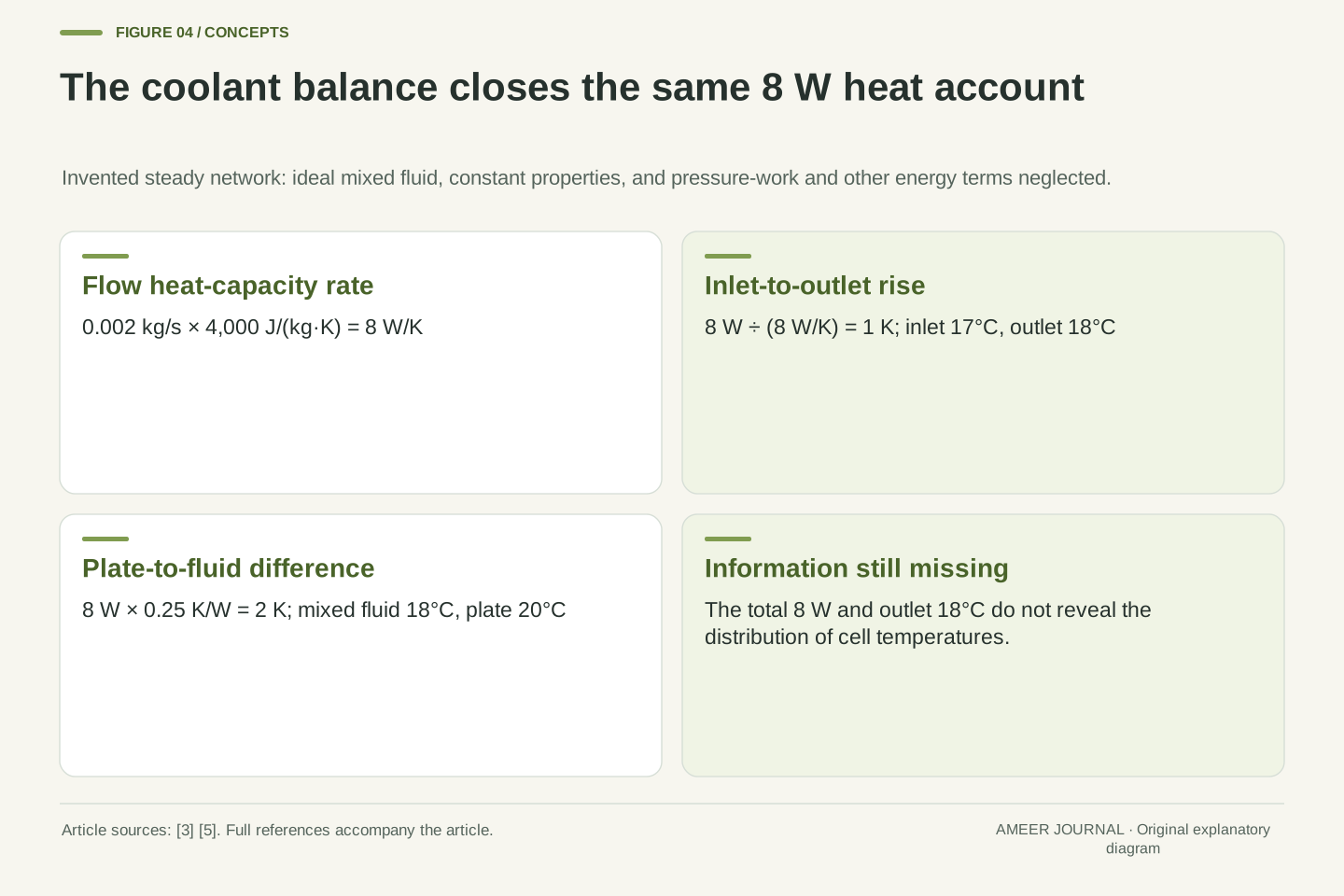
We can now complete the route from the cells to the fluid. Let coolant enter the invented system at 17°C. It flows into an ideal perfectly mixed region, so the fluid leaving has the same temperature as that region. Give the flow a mass rate of 0.002 kilograms per second and a constant specific heat of 4,000 joules per kilogram per kelvin. These are model inputs, not a coolant recommendation.
Multiplying the two values gives 8 watts per kelvin. At steady conditions, absorbing 8 watts therefore raises this flowing fluid by 1 kelvin between inlet and outlet. It leaves at 18°C. This simple account neglects pressure-work and other energy terms; MathWorks presents the more general steady-flow balance and distinguishes coolant inlet from outlet temperatures. [5]
Finally, put a thermal resistance of 0.25 kelvin per watt between the common plate and the mixed fluid. Carrying 8 watts requires a 2-kelvin difference, placing the plate at 20°C. [3] That closes the earlier examples: A, B and C all send 8 watts to the plate, all produce the same coolant outlet and all share the same plate temperature. The fluid’s overall energy gain has not identified how the heat was distributed between cells.
Complete the steady network with inlet T_in = 17°C, mass flow ṁ = 0.002 kg/s and constant specific heat c_p = 4,000 J/(kg·K). The coolant node is ideally mixed, with T_out equal to its node temperature. Neglect pressure-work, kinetic and potential-energy differences, other heat inputs and coolant storage change. The resulting flow balance is Q = ṁc_p(T_out − T_in); the referenced documentation retains a pressure term in its more general expression. [5]
The heat-capacity flow rate is ṁc_p = 8 W/K. With Q = 8 W, the inlet-to-outlet rise is 1 K and T_out = 18°C. This is distinct from the cell heat capacity C = 240 J/K: one is a rate associated with continuously flowing mass; the other is a storage coefficient for a fixed node. Confusing them would also confuse the time dimensions in the calculation.
Let the plate-to-mixed-coolant resistance be R_p = 0.25 K/W. Then T_p − T_out = QR_p = 2 K, making T_p = 20°C. [3] Each of A, B and C satisfies the same total flow balance and this same plate condition. The model uses a mixed fluid node, not an unsupported identification of a real channel’s outlet with its spatially averaged coolant temperature.
More flow changes one part of the temperature difference
Change just the mass flow to 0.004 kilograms per second, twice its earlier value. Keep the inlet, generated heat, fluid specific heat and every resistance fixed. The flow now carries 16 watts per kelvin. The same 8 watts raises it by only half a kelvin, so the outlet is 17.5°C. The plate remains 2 degrees above the mixed fluid and is now at 19.5°C.
For case A, the cell-to-plate differences remain 12 and 4 degrees. Its cells become 31.5°C and 23.5°C, each half a degree cooler than before. The 8-degree spread is unchanged. Doubling the flow has halved the fluid’s inlet-to-outlet rise in this calculation; it has not halved either absolute cell temperature or either cell-to-plate difference.
The fixed-resistance condition is essential. Keeping every effective resistance fixed in a real circuit would need justification, so this is a sensitivity calculation for the declared model. The example still reveals a useful reading rule: a smaller coolant temperature rise does not necessarily mean less heat was removed. Here the rise halves while the mass flow doubles, leaving the heat-transfer rate unchanged. Read the flow rate and temperature rise together. [5]
A controlled model sensitivity doubles ṁ to 0.004 kg/s while holding P_A + P_B = 8 W, c_p, T_in and all thermal resistances fixed. The flow capacity rate becomes 16 W/K. Thus T_out = 17 + 8/16 = 17.5°C, and T_p = 17.5 + 8(0.25) = 19.5°C. The energy balance changes the coolant rise without changing the total heat rejected. [5]
For state A, P_AR_A = 12 K and P_BR_B = 4 K remain unchanged. Consequently, T_A = 31.5°C and T_B = 23.5°C. Both shift by −0.5 K, while their difference remains 8 K. A lower fluid temperature translates the two node temperatures in this model; it does not remove the unequal branch offsets that produced the span.
Holding effective resistances constant isolates the flow-capacity term. It should not be read as a general prediction for a modified cooling circuit: actual fluid properties and heat-transfer behaviour can depend on operating conditions. MathWorks explicitly distinguishes its constant-property calculations from a simulation with pressure- and temperature-dependent properties. [5] The transferable inference is narrower: outlet rise alone cannot establish heat rate when flow or fluid properties differ. The product ṁc_pΔT and the stated energy boundary are required.
Follow the changing spread rather than only the mean
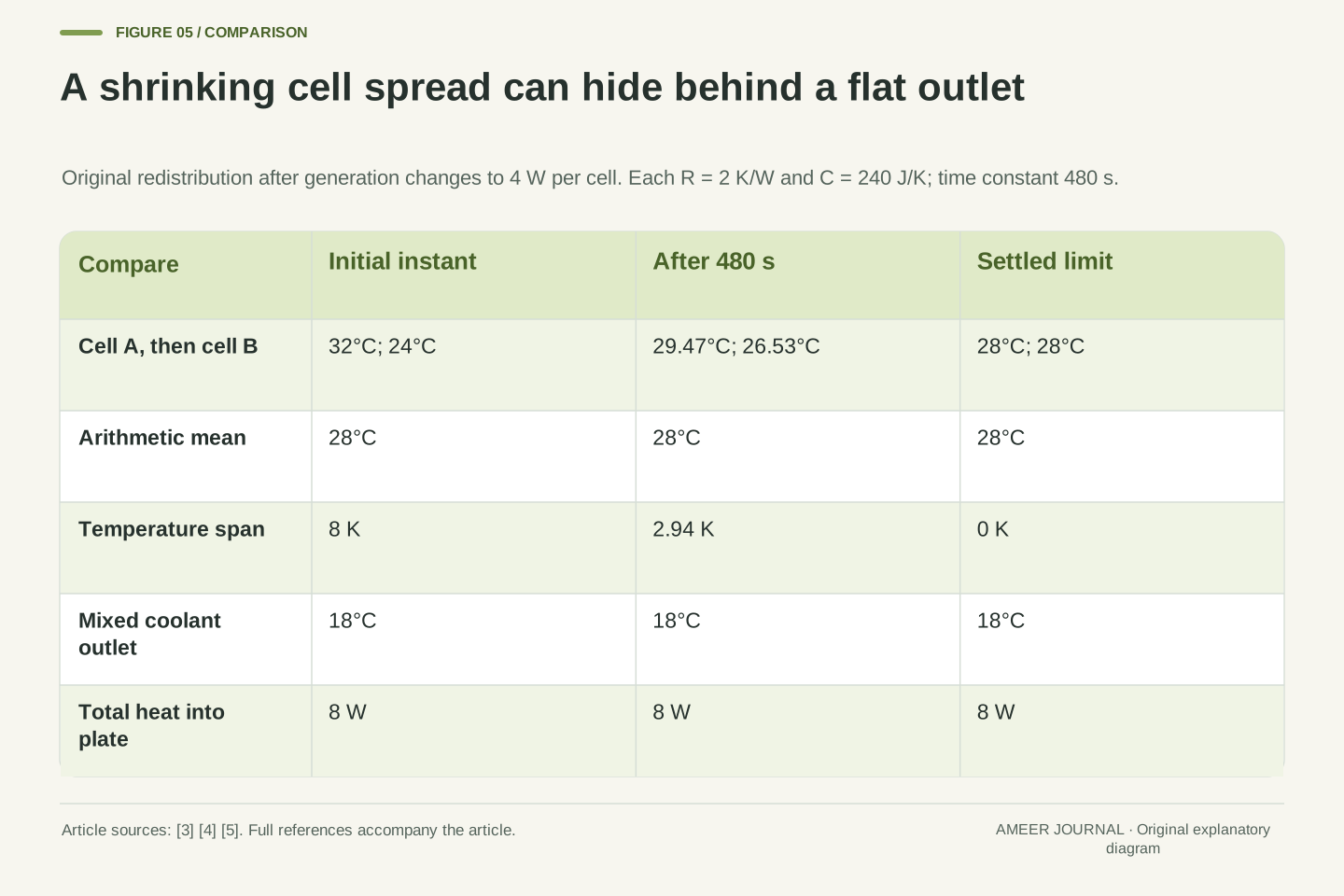
The model also tells us how the cells approach their common final temperature. Their resistance multiplied by their heat capacity gives a time scale of 2 × 240 = 480 seconds. The hotter cell starts 4 degrees above 28°C and the cooler cell 4 degrees below it. After 480 seconds, each remaining difference is about 1.47 degrees. The cells are therefore about 29.47°C and 26.53°C.
The average is still 28°C, but the spread has fallen from 8 degrees to about 2.94 degrees. After 960 seconds, the temperatures are about 28.54°C and 27.46°C. Their final limit is 28°C each. This pattern follows from the constant resistance and heat-storage equations, rather than a measured trace or a claim about how quickly a particular EV responds. [3][4]
There is no direct heat path from one cell to the other in this model. Both keep transferring heat toward the plate. The warmer cell loses some stored energy because it initially removes more than it generates; the cooler cell retains some of its newly generated energy. Doubling both heat capacities would double the time scale to 960 seconds without changing the final steady temperatures. More storage slows a change; it does not create a permanent route for removing heat.
With the common plate held at its consistent 20°C solution, each node satisfies C dT_i/dt = 4 − (T_i − 20)/R. Its equilibrium is 28°C and its time constant is τ = RC = 480 s. For t ≥ 0, T_A = 28 + 4 exp(−t/480) and T_B = 28 − 4 exp(−t/480), with temperatures in °C and t in seconds. Their span is 8 exp(−t/480) K. [3][4]
At t = 480 s, the values are approximately 29.4715°C and 26.5285°C; the span is 2.9430 K. At 960 s they are 28.5413°C and 27.4587°C. Relative to a 20°C reference, initial stored energies are 2,880 J and 960 J, tending to 1,920 J each. Total stored energy stays 3,840 J: the changes −960 J and +960 J cancel.
Those opposite changes do not imply direct transfer from A to B. Both branch flows stay toward the cooler plate; their rates converge to 4 W from opposite sides. The changing allocation of generation and outgoing heat accounts for each storage change. If both C values become 480 J/K with the other assumptions retained, τ becomes 960 s while the same steady temperatures remain. Thermal capacity controls response and stored energy; steady rejection depends on generation, paths and boundary conditions.
Different evidence answers different thermal questions
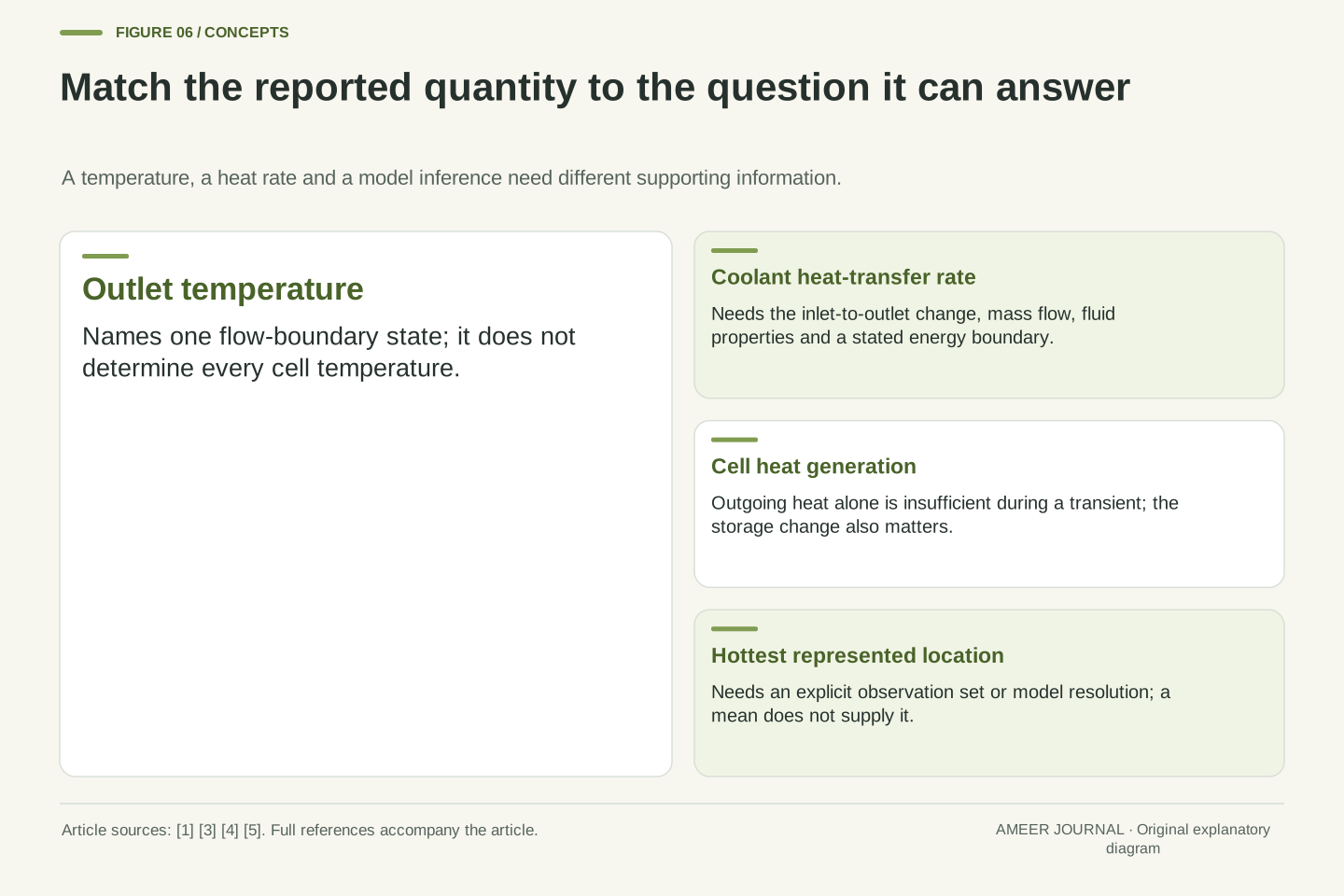
A temperature map asks where temperatures differ. A heat-generation measurement asks how quickly energy is being produced under the conditions being examined. A system model connects those observations through stated paths and storage. These tasks support one another, but they are not interchangeable. NLR describes combining calorimetry with thermal imaging and assessing behaviour from cells through integrated systems. [1]
This matters when a cooling claim moves from one component to a whole battery. A useful material property does not by itself describe every interface, every source of heat or the final distribution. SwRI describes work across components, subsystems and complete applications. NLR’s public 2024 paper abstract also reports module-interconnect heat and temperature non-uniformity associated with cooling arrangement. [2][6] Those details explain why the boundary of the assessment matters.
Our two-cell calculation deliberately omits interconnect sources and internal cell gradients. Adding them would add unknowns, not magically make the outlet a complete description. When reading an engineering report, look for the locations represented, the operating conditions, the heat sources included and the comparison between model and observations. A measured maximum, a predicted maximum and a whole-pack average should keep their own labels even when their numerical values happen to match.
Temperature-field evidence, calorimetry and system modelling constrain different parts of the thermal problem. A temperature distribution constrains state variables at represented locations; calorimetry can characterize heat generation under specified conditions; a model relates sources, paths, storage and boundaries. NLR’s program explicitly combines these approaches across assembly levels. [1] Agreement between two reported numbers is weaker evidence than an identified, condition-matched relationship between them.
The public 2024 NLR abstract describes cell heat-generation characterization, additional module-interconnect heat and non-uniformity associated with cooling arrangements. [6] Only that actual abstract is used here, not unseen numerical results or a reconstructed pack model. SwRI likewise describes component-through-system evaluation. [2] These sources support the need to identify the assessment level; they do not supply the invented two-cell parameters.
Our lumped nodes remove spatial resolution inside cells, omit interconnect heat and use fixed effective properties. Those reductions make the non-uniqueness proof transparent, but would require separate justification in a predictive model. A real comparison would need the relevant operating state and observation coverage, rather than treating a good fit to an outlet channel as proof that every internal temperature was reproduced. The distinction is between what the evidence directly constrains and what the model additionally assumes.
Read a thermal claim as a set of connected quantities
Begin with the noun beside the number: coolant inlet, coolant outlet, plate, cell location, average or maximum. Then ask whether the condition is steady or changing. In the examples here, 18°C at the outlet and 28°C as the average fit several different interiors. Adding a maximum distinguishes some possibilities; adding information about generation or paths distinguishes others. Each added fact has a specific job.
Next, keep the energy account intact. A fluid temperature rise needs a flow rate and suitable fluid-property information before it becomes a heat-transfer rate. A cell temperature difference needs a path model before it becomes an outgoing heat rate. During a change, heat storage separates that outgoing rate from the cell’s internal generation. The equations used above make those missing links explicit. [3][4][5]
The practical benefit is better interpretation of published specifications, technical explanations and temperature charts. A lower coolant reading can be useful evidence without describing the whole battery. A constant average can coexist with a shrinking spread. A larger heat capacity can slow movement without changing the final temperature. Asking which quantity changed, where it was measured and which conditions stayed fixed turns a thermal headline into a question that the available evidence can actually answer.
Preserve the chain of definitions: observable location, aggregation rule, time condition, thermal boundary and inferred quantity. A mean is a summary over a specified set; a maximum depends on coverage; an outlet reading belongs to a flow boundary. The examples demonstrate two separate ambiguities: identical aggregates can hide different cell extremes, and identical cell temperatures can arise from different combinations of generation and resistance.
For inference, use only the relation justified by the boundary. The branch equation gives outgoing Q from ΔT and known R. The storage equation connects generation P to Q and C dT/dt. The simplified coolant equation connects total Q to ṁc_pΔT under the stated exclusions. [3][4][5] Applying one relation without its missing variables does not turn a partial temperature record into a complete thermal characterization.
A useful report therefore keeps source distribution, heat paths, thermal capacity, coolant conditions and measurement coverage visible. Our constructed trajectory has constant mean, plate temperature, outlet temperature and total heat rejection while its cell spread decays. That is the central result: aggregate thermal stability and internal thermal uniformity are different statements. Assessing one does not automatically establish the other, even with perfect instruments and internally consistent arithmetic.
Sources & further reading
Explore the references behind this guide. External pages may change after our review.
- Energy Storage Thermal Management
| Transportation and Mobility Research | NLRNational Laboratory of the Rockies · Accessed 7 Nov 2026
- Cool Battery Tech | Southwest Research InstituteSouthwest Research Institute · Accessed 7 Nov 2026
- Thermal Resistance - Constant resistance in thermal systems - MATLABMathWorks · Accessed 7 Nov 2026
- Thermal Mass - Mass in thermal systems - MATLABMathWorks · Accessed 7 Nov 2026
- EV Battery Cooling System Design - MATLAB & SimulinkMathWorks · Accessed 7 Nov 2026
- Li-ion Battery Thermal Characterization for Thermal Management Design: Article No. 136
- National Laboratory of the RockiesNational Laboratory of the Rockies research publication record · Accessed 7 Nov 2026
Article updated 7 Nov 2026.
Found something we should revisit?
Good explanations get better with thoughtful feedback.