A charging timer can obey its selected hours perfectly and still leave an energy target unfinished. The timer decides when charging is permitted. The target asks how much energy must arrive before the car leaves. A cheaper unit price helps with the bill only after enough usable charging time and power are available. DOE’s managed-charging guidance treats operating schedules, electricity prices and power limits as separate inputs to that decision. [1]

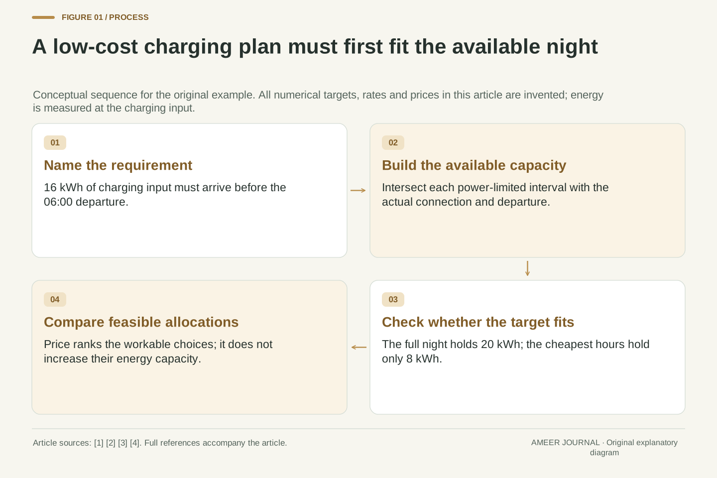
We will examine one invented night, from arrival at 22:00 to departure at 06:00. The charging plan needs 16 kilowatt-hours from the electricity supply. Available power and price change during the night. First we will check whether the target is possible, then find the cheapest feasible allocation, and finally move the departure time. Every power, price and energy value is supplied for this example; no car, household tariff or scheduling product was tested.

This is a different question from whether a charger can replace a week’s driving energy. Here the challenge is placing a fixed energy requirement into particular hours. Some residential tariffs charge different rates at different times, but that is a feature of the actual tariff, not a universal rule that nighttime electricity is cheap. [3][4]

Charging feasibility and energy-cost minimization are separate problems. Feasibility asks whether a permitted power trajectory can deliver a required energy quantity before a deadline. Optimization asks which feasible trajectory has the smallest stated cost. DOE’s managed-charging discussion explicitly distinguishes vehicle operations, time-dependent rates, equipment capacity and building loads. [1] A low-price interval is therefore an input to the problem, not proof that its energy requirement can be met.

Our original deterministic model uses an eight-hour connection from 22:00 to 06:00 and a 16 kWh grid-input target. Four piecewise-constant slots have known power caps and marginal energy prices. Charging can be interrupted and continuously adjusted within each cap; sufficient permitted storage headroom is assumed. All numbers are invented, and no controller, vehicle or tariff calculation service was run. Ordinary elapsed hours are used throughout.

The primary objective will be minimum energy charge, subject to meeting the target. We will separately calculate earliest completion and latest feasible start, because those are different properties. Residential time-of-use pricing is tariff-dependent; EIA distinguishes retail arrangements from continuously changing wholesale supply costs. [3][4] Our price table is a mathematical input, not a statement about either market today.

Kilowatts describe a rate; kilowatt-hours describe energy delivered over time. A constant two-kilowatt input for two hours supplies four kilowatt-hours. [2] Every power and energy entry in our timetable refers to the charging input from the supply. The target is therefore 16 supply kWh. Keeping that boundary fixed lets us compare the target with available energy and multiply delivered energy by a price per supply kWh.

If we also want a battery-side interpretation, stipulate a constant conversion factor of 0.80 for this example. Then 16 input kWh corresponds to 12.8 kWh added to the modeled stored energy. Conversely, a 12.8 kWh stored-energy requirement would need 12.8 divided by 0.80, or 16 input kWh. The factor is invented and includes the entire modeled difference between input and addition; it is not a measured charging efficiency.

We will do the scheduling in the input column. That avoids charging for 12.8 kWh while actually planning to draw 16. It also avoids treating a battery percentage as an energy quantity without knowing its meaning. The required addition is taken as already established and allowed; the timetable is not choosing a recommended charge level or predicting how far the car will travel.

Let E_g be charging energy drawn at the grid-input boundary. With constant power P_g over duration Δt, E_g=P_gΔt; kW multiplied by hours gives kWh. [2] The model requirement is E_g=16 kWh. Slot prices are dollars per kWh at this same input boundary. Neither the numerator in the energy constraint nor the billed-energy variable changes definition partway through the calculation.

For an optional stored-energy interpretation, define a constant aggregate factor η=0.80 and ΔE_b=ηE_g. Thus E_g=16 kWh gives ΔE_b=12.8 kWh. If the requirement were supplied as ΔE_b=12.8 kWh, the corresponding input target would be ΔE_b/η=16 kWh. This is an assigned mapping, with no additional unmodeled consumption outside it, rather than a component-efficiency measurement or a state-of-charge conversion.

A constant η preserves the ordering of slots by cost per stored kWh because every grid price is divided by the same factor. That observation would change if conversion varied by slot. Here it simply justifies performing the whole allocation at the input boundary. Battery headroom, the required addition and its permission are premises; the exercise does not infer them from a percentage display or a nominal pack capacity.

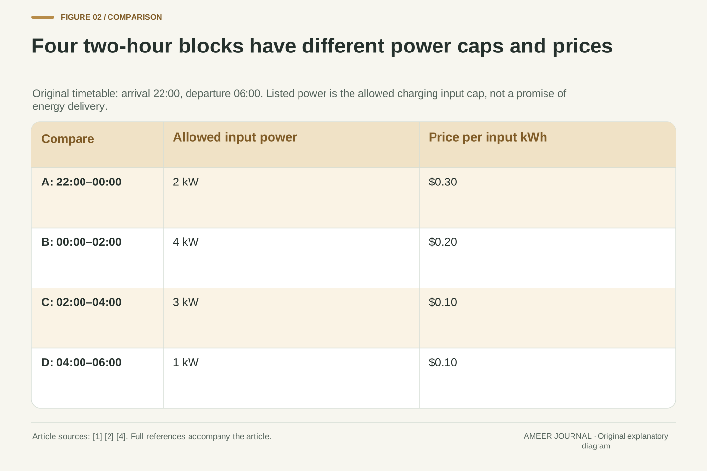
Divide the night into four two-hour blocks. Call 22:00–00:00 block A, 00:00–02:00 B, 02:00–04:00 C and 04:00–06:00 D. The allowed charging powers are respectively 2, 4, 3 and 1 kW. Their invented prices are $0.30, $0.20, $0.10 and $0.10 per input kWh. The lower price in the last two blocks does not imply that their available charging power is higher.

One way to construct those changing caps is to give a fictional site an aggregate six-kilowatt ceiling. Its other loads use 4, 2, 3 and 5 kW in the four blocks, leaving 2, 4, 3 and 1 kW for charging. Also stipulate a four-kilowatt charging-equipment and vehicle ceiling. This is a scheduling illustration of the building-load and power-limit considerations in managed charging, not an electrical installation calculation. [1]

Multiply each allowed rate by its two usable hours. The blocks can contribute at most 4, 8, 6 and 2 kWh. [2] These are capacities, not promises that all that energy will be delivered. A schedule may use less, stop when the target is reached, or leave an entire block unused. The capacity column is what tells us how much room each part of the night provides.

Index slots A through D with intervals [22:00,00:00], [00:00,02:00], [02:00,04:00] and [04:00,06:00]. Their durations are all 2 h. Define charging caps P̄=(2,4,3,1) kW and marginal prices p=(0.30,0.20,0.10,0.10) dollars/kWh. A chosen slot energy e_i must satisfy 0≤e_i≤P̄_iΔt_i. No minimum operating power, session-start penalty or coupling between adjacent slots is included.

The caps can be reproduced from a stipulated aggregate ceiling G=6 kW, background loads b=(4,2,3,5) kW and joint charging ceiling P_max=4 kW: P̄_i=min(P_max,max(0,G−b_i)). DOE describes power ceilings and adaptation to building loads as managed-charging considerations. [1] The scalar G is an invented scheduling constraint, not a panel rating, wiring specification or code-based continuous-load limit.

The corresponding energy-capacity vector is C=(4,8,6,2) kWh. This multiplication uses actual usable duration, so a deadline inside a slot will change that slot’s capacity. [2] Distinguish C_i, the maximum available amount, from e_i, the amount selected. The model allows any intermediate amount by varying power or using part of an interval, while retaining the stated upper bound.

Across the complete connection, the four capacities add to 4+8+6+2=20 kWh. The 16 kWh target can therefore fit somewhere in the night under our rules. We have not yet decided where to place it or what it will cost. This first check answers a simpler question: is there enough possible delivery before departure, even if we use expensive hours?

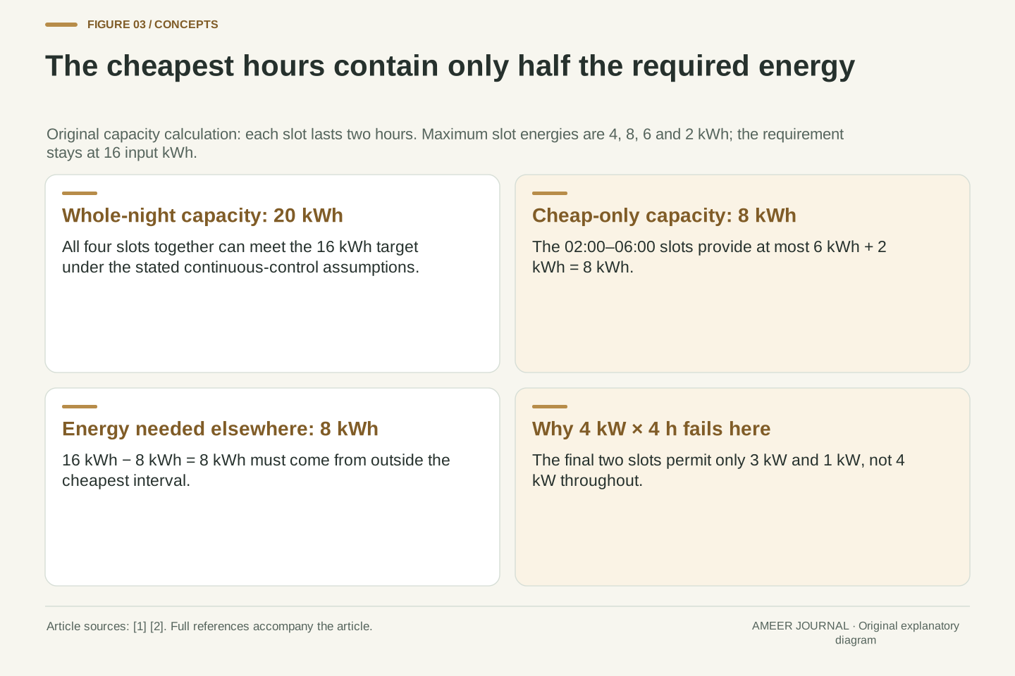
Now restrict charging to the cheapest period, 02:00–06:00. Block C can provide six kWh and block D two, giving only eight. That is half the required sixteen. Multiplying the four-kilowatt equipment ceiling by all four cheap hours would give sixteen, but it would assume power that the slot constraints do not allow. The charging opportunity is limited by the usable power in each hour, not by the largest number elsewhere in the plan. [1][2]

Because the full night is feasible and the cheap-only window is not, some higher-rate energy is necessary. This does not yet tell us how much should come from each higher-rate block. It tells us that a plan advertising the lowest unit price while supplying only eight kWh cannot be compared fairly with a plan that actually supplies the target. Both cost and completion need to describe the same requirement.

For the stated independent continuous bounds, feasibility is equivalent to E_req≤ΣC_i, with a nonnegative target and sufficient storage headroom. Necessity follows because no slot can exceed its capacity. Sufficiency follows by assigning energy successively to available capacities until the target is filled; continuous interruptibility permits the last slot to be only partly used. Here ΣC_i=20 kWh≥16 kWh, so a feasible allocation exists.

Restricting eligible slots to C and D reduces the maximum to 6+2=8 kWh. Therefore the cheap-only policy is infeasible for the same 16 kWh requirement. The shortcut 4 kW×4 h=16 kWh uses the equipment ceiling as though it were the available power throughout both slots. The declared caps are instead 3 kW for two hours and 1 kW for two hours. Their energy integral is eight kWh. [1][2]

At least eight kWh must consequently be assigned outside the cheapest interval. This lower bound follows from energy capacity before any optimization argument. Feasibility also depends on the deadline: unused capacity after departure cannot compensate for a deficit before it. The current twenty-kWh total belongs specifically to the complete 22:00–06:00 availability, not to every possible start or departure within that night.

Use all eight kWh available in the two ten-cent blocks. Eight kWh still need a home. Block B can supply exactly that amount at twenty cents per kWh, so the thirty-cent block A can remain unused. The allocation is therefore A: zero, B: eight, C: six and D: two kWh. The energy charge is $1.60+$0.60+$0.20=$2.40 for the complete sixteen-kWh target.

Why is this the cheapest choice under our assumptions? Suppose a plan buys some energy at thirty cents while leaving room in the twenty-cent block. Moving one kWh into that unused room keeps the delivered total unchanged and saves ten cents. The same reasoning favors unused ten-cent capacity over twenty-cent energy. Once all useful cheaper room is filled, no such saving remains. This is our calculation using the time-dependent pricing idea described by DOE and EIA. [1][4]

In this particular case, B, C and D must all run at their allowed rates for their full durations to supply sixteen kWh without A. The last energy arrives at 06:00. Equal prices do not generally force one exact schedule, but here both cheap blocks are fully needed. The result minimizes the stated energy charge; it has not selected the earliest completion time or added a spare-time requirement.

Minimize J=Σp_i e_i subject to Σe_i=16 kWh and 0≤e_i≤C_i. All prices are positive, and there is no benefit assigned to exceeding the target, so equality is appropriate. Filling the ten-cent capacity first supplies e_C=6 and e_D=2 kWh; the remaining eight fits e_B=8 kWh. Thus e=(0,8,6,2) kWh and J=0.20×8+0.10×6+0.10×2=$2.40.

An exchange argument establishes optimality. If a feasible allocation uses energy in a higher-price slot while a lower-price slot has unused capacity, transfer a sufficiently small equal amount between them. The total and bounds remain satisfied while cost falls by the price difference times the transferred energy. Repeating this removes every such opportunity. The proof relies on linear marginal pricing and uncoupled capacity constraints, consistent with our declared simplification of the managed-charging problem. [1][4]

Although C and D have equal prices, this target requires their combined full capacity plus all of B. The resulting slot-energy vector is unique for these inputs. Charging at the caps in B, C and D completes at 06:00. This uniqueness is specific to the target and capacities; it is not a general property of time-of-use schedules or a claim about how any commercial controller resolves equal-price alternatives.

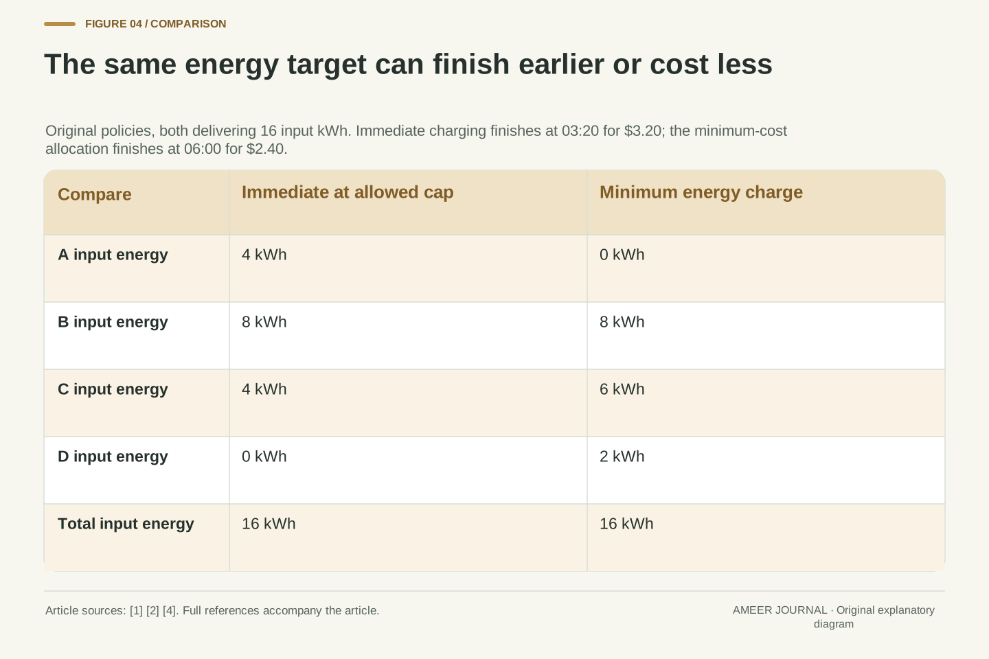
For a second policy, begin charging at the allowed maximum as soon as the fictional car arrives. Block A supplies four kWh, and B adds eight, bringing the total to twelve at 02:00. Four more kWh are needed. At C’s three-kilowatt rate, that takes one hour and twenty minutes. The target is reached at 03:20, and charging stops before D begins.

This immediate policy costs four times thirty cents, eight times twenty cents and four times ten cents: $1.20+$1.60+$0.40=$3.20. It supplies exactly the same sixteen kWh as the $2.40 allocation. The cheaper plan saves eighty cents, which is 25% of this immediate plan’s charge. These are two calculated outcomes from one invented table, not expected savings on a household bill.

The immediate policy does have another property: it finishes two hours and forty minutes before departure. The cheapest policy finishes at departure itself. Which property matters depends on the requirement being evaluated. DOE separates operating needs from cost control for this reason. [1] A price comparison should not hide the completion times, and an early-finish comparison should not imply that the energy charges were equal.

The immediate-at-cap policy fills A and B, supplying 4+8=12 kWh by 02:00. Its remaining four kWh requires 4/3 h in C, so completion is 03:20. The chosen energies are e_immediate=(4,8,4,0) kWh. This is also the earliest feasible completion under the supplied caps, because it uses every available earlier opportunity until the target is met.

Its linear energy charge is J_immediate=0.30×4+0.20×8+0.10×4=$3.20. Relative to J_min=$2.40, the absolute difference is $0.80 and the reduction measured against immediate charging is 0.80/3.20=0.25. The denominator is the immediate policy’s charge, not the minimum charge or a complete monthly electricity bill. Fixed fees, taxes, demand charges and other terms remain outside the model.

The two policies optimize different properties: using maximum power immediately minimizes completion time, while allocating energy by price minimizes the declared charge. DOE’s discussion distinguishes uncontrolled immediate charging from managed timing and power choices. [1] Our construction gives a concrete instance of that difference. Neither result alone establishes resilience to changed conditions; the cheap solution has no idle time remaining between its midnight start and its six-o’clock completion.

Start at the departure end of the timetable. The final two hours can provide two kWh. Add the preceding block’s six and we have eight. Add all eight from midnight to 02:00 and we reach sixteen. Therefore midnight is the latest possible start for this target and deadline, provided the allowed power is used continuously afterward. The earlier 22:00–00:00 block is unnecessary for that particular feasible plan.

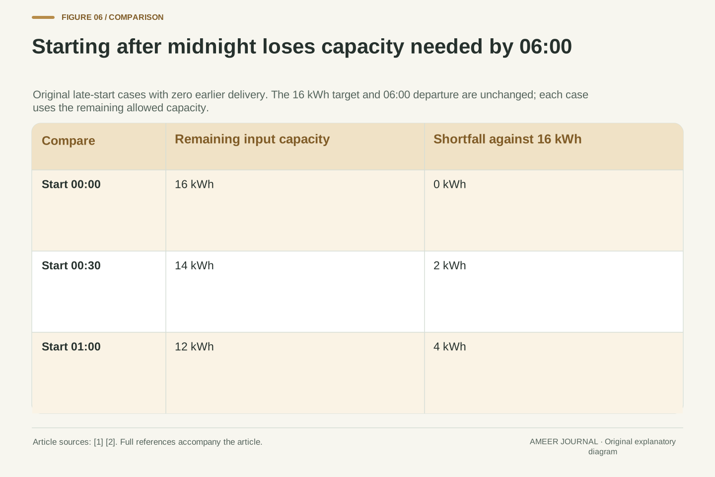
Now delay the start to 00:30 with nothing charged earlier. Only one and a half hours remain in B, so it can provide six kWh instead of eight. Add C’s six and D’s two and the remaining night can supply fourteen. The target is two kWh short. A 01:00 start leaves only four kWh in B and twelve overall, making the shortfall four. A six-o’clock finish goal cannot create the lost capacity.

The cheapest plan and the latest feasible start happen to agree here because the lower-price blocks sit later and their capacities fit the target exactly. That is a feature of this table. Moving the prices while keeping the power limits unchanged could change the cheapest allocation without changing the latest feasible start. Price chooses among workable schedules; the physical delivery constraint defines which schedules are workable. [1][2]

For a candidate start a and departure d, define available energy C(a,d) as the integral of the permitted charging cap over their overlap with the connection. Working backward from 06:00, suffix capacities are 2 kWh from 04:00, 8 kWh from 02:00 and 16 kWh from 00:00. Consequently a_latest=00:00 for the original sixteen-kWh requirement. Any positive delay after midnight removes some needed capacity.

With a=00:30, B’s remaining duration is 1.5 h and its capacity is 4 kW×1.5 h=6 kWh. The total becomes 6+6+2=14 kWh, leaving a two-kWh deficit. Starting at 01:00 leaves 4+6+2=12 kWh and a four-kWh deficit. Both cases assume zero earlier delivery; they are not descriptions of a paused session that already accumulated energy before the selected start.

Latest-start feasibility depends on target, availability and caps, not on prices. Cost optimization additionally depends on the price vector. Their coincidence in the main case is therefore contingent: a different price ordering could favor early charging while the same capacity integral still permits a midnight start. DOE’s separation of operational schedules and utility rates is useful here because changing one does not automatically change the other. [1]

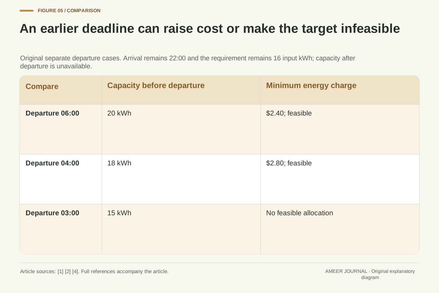
Change the departure to 04:00 while leaving arrival, target and the earlier blocks unchanged. Block D is gone. A, B and C together can still supply eighteen kWh, so the sixteen-kWh target remains possible. The cheapest choice takes six from C, eight from B and the remaining two from A. Its cost is $0.60+$1.60+$0.60=$2.80. The earlier departure costs forty cents more in this particular comparison.

Two kWh in A takes one hour at its two-kilowatt limit. A schedule can therefore begin at 23:00, use the final hour of A, then use all of B and C to finish at 04:00. Midnight is no longer a feasible start: the two later blocks together hold only fourteen kWh. Reusing the previous start time without updating the departure would keep a familiar setting while losing the energy it was meant to provide.

Move departure earlier again, to 03:00. Now only the first hour of C is available, contributing three kWh. Even starting immediately at 22:00 gives four plus eight plus three, or fifteen kWh. No permitted allocation meets sixteen. The important boundary falls inside a block, so counting the whole two-hour block would be wrong. These changed cases show why operating-time changes require the schedule to be reconsidered. [1]

For a 04:00 deadline, the capacity vector becomes (4,8,6,0) kWh and its total is 18 kWh. Re-solving the same linear objective yields e=(2,8,6,0) kWh: all ten-cent capacity, all twenty-cent capacity and two thirty-cent kWh. The minimum charge is 0.30×2+0.20×8+0.10×6=$2.80. This is a new optimum under a changed constraint, not the original allocation with its final segment silently omitted.

Backward accumulation reaches fourteen kWh from midnight to 04:00. Two more kWh requires one hour of A, establishing 23:00 as the latest start under the original caps. Starting then at 2 kW, followed by the full B and C caps, meets the target exactly. Both the cost and the latest-start answer have changed even though the energy requirement and arrival time remain fixed.

For a 03:00 deadline, intersect C with the available interval before calculating capacity. Its duration is one hour, so C contributes 3 kWh and total capacity is 4+8+3=15 kWh. The feasible set is empty for a sixteen-kWh target. Neither a different price-ranking algorithm nor a finish-by label can repair that mathematical deficit. Updated arrival/departure inputs are part of the schedule-management problem described by DOE. [1]

A start-time setting and a finish-by setting do different jobs. One selects when charging begins. The other gives a target time from which a controller may estimate a required start. As one documented example, the retrieved UK-English Model 3 manual distinguishes Start at from End by and describes calculating a start time for an end-only schedule. It also describes immediate charging in a specified insufficient-time case. [5]

That is a particular owner-manual description, not a claim that every car or wall unit uses the same rules. Our four-slot calculation is not an account of Tesla’s algorithm. The useful distinction is between the requested outcome and the inputs used to estimate when work must begin. If the car is connected late or the available power differs, an earlier estimate may no longer fit the actual opportunity.

In our original example, a midnight start works only because sixteen input kWh remain deliverable before 06:00. At 00:30, starting immediately is the best possible response for meeting that deadline, but the limit is fourteen. A controller can change a schedule within its permitted choices; a label on the screen cannot make a constrained fourteen-kWh opportunity supply sixteen. The target and the achievable result should remain separate in any interpretation of the display.

Scheduling interfaces may expose an action time or a completion objective. The retrieved UK-English Model 3 manual provides a bounded example: an End by configuration without Start at uses an estimated start, whereas Start at alone begins at that time and continues toward the charge limit. The manual also names an insufficient-time condition for immediate charging. [5] These semantics belong to that document, not every charging system.

Our optimization is independent of that implementation. A completion-time request does not determine the realized power function, and an estimated start inherits assumptions about required energy and available delivery. In the toy model the latest valid estimate is midnight. If connection occurs at 00:30 with no prior energy, integrating the maximum permitted rate gives fourteen kWh, so the sixteen-kWh target is infeasible even with immediate action.

Separate requested deadline, estimated start, actual connection and actual delivery when reading a scheduling record. Those quantities can disagree without being the same kind of error. A late connection changes the available interval; a different power cap changes its capacity; a revised target changes the required integral. The software’s precise handling requires its own documentation, while the energy shortfall follows directly from the stated constraints.

A useful update starts with the amount still needed, not the original target in isolation. If eight input kWh have already arrived, the sixteen-kWh target has eight remaining. Compare that remainder with the power and time still available. Past energy counts toward the target; past unused hours do not remain available. DOE describes dynamic management as responding to changes in operating schedules, equipment capacity and building loads. [1]

Consider a separate change known before arrival: other loads during 04:00–06:00 will use 5.5 kW instead of five. Under the same six-kilowatt aggregate ceiling, D’s charging cap falls from one to half a kilowatt. Its two-hour capacity falls from two to one kWh. The cheapest revised allocation is A: one, B: eight, C: six and D: one, costing $0.30+$1.60+$0.60+$0.10=$2.60.

Now suppose that change becomes known only at midnight, after A has passed unused. The remaining blocks hold fifteen kWh, so the unchanged sixteen-kWh target cannot be met. Buying the extra kWh earlier would have worked if the information had been available then; it is no longer an available decision. This is why total spare capacity at arrival and spare capacity later in the night are different things.

At an update time t, the residual constraint is E_remaining=E_req−E_delivered(t), using compatible energy boundaries. Feasibility then compares that remainder with the integral of future permitted power. Previously delivered energy reduces the requirement, whereas previously unused capacity cannot be carried forward. This is the mathematical reason a dynamic plan must use its actual history along with revised forecasts, as motivated by DOE’s description of adaptive management. [1]

In a separate deterministic sensitivity case, set the final background load to 5.5 kW. The same cap formula gives P̄_D=0.5 kW and C_D=1 kWh. If known before 22:00, the optimal energy vector is (1,8,6,1) kWh and its charge is $2.60. One thirty-cent kWh replaces one ten-cent kWh, explaining the twenty-cent increase over the original $2.40 optimum.

If the revised cap becomes known at 00:00 after zero delivery in A, future capacity is only 8+6+1=15 kWh. The sixteen-kWh residual target is infeasible. This comparison changes the time at which information is available while keeping the revised physical caps identical. It demonstrates the value of earlier available capacity without assuming a particular forecast distribution, automatic response or universally sufficient reserve margin.

The cheap-capacity rule worked because every delivered kWh could move independently between eligible blocks, subject to their limits. Prices were charged per input kWh, and stopping or restarting carried no extra cost. A real plan with another charging rule or a different bill structure needs those details included. For example, a charge based on the highest power during a period would introduce something beyond our simple sum of energy times price.

The same care applies to capacity. Our fictional equipment could supply any rate up to each cap, and the target fit within allowed storage. If a particular system permits only certain operating levels, or its available delivery changes with other conditions, the table must represent that behavior. AFDC describes timers and communications as features of some home equipment; their presence does not establish every control capability assumed in this mathematical example. [3]

A readable schedule therefore keeps its energy boundary, arrival, departure, available power and marginal price together. It states the selected energy in each block and checks the total before displaying a cost. Our answers then stay understandable: cheap-only charging supplies too little; the cheapest feasible plan supplies sixteen kWh for $2.40; and changing the deadline or losing a slot can change the answer. Those conclusions come from the complete timetable.

The exchange proof requires a linear separable objective and independent interval-capacity constraints. Session charges, minimum operating power, state-dependent acceptance, varying conversion, inter-slot restrictions or a peak-demand term can alter the feasible set or objective. Such additions require a corresponding model; the current solution should not be promoted into a universal scheduling algorithm. A hypothetical demand charge, for example, depends on an extremum rather than just the energy integral.

Our scalar caps are known inputs, the constant conversion factor has one declared boundary, and energy can be continuously allocated or interrupted. AFDC’s discussion of optional timers and communications does not certify those exact capabilities for arbitrary equipment. [3] Likewise, a retail tariff must supply the actual price rules; wholesale variation alone does not establish the marginal rate paid by a household. [4] The model is useful because these conditions are visible.

An interpretable result reports target energy, eligible intervals, cap-derived capacities, chosen energies, completion time and the cost definition. Feasibility is checked before comparing objective values. The original example then yields distinct, reproducible answers for minimum charge, earliest completion, latest start, earlier departure and changed future capacity. No single overnight label carries all those meanings; the event times and energy constraints establish which conclusion is justified.