What you’ll take away
- Peak power is one point; an equal-energy comparison needs the entire relevant charging interval.
- A power-versus-time chart and a power-versus-state-of-charge chart require different calculations.
- Use total energy divided by a defined elapsed time, and state whether pauses are included.
- Equal percentage windows can represent different energy amounts when usable capacities differ.
- A journey decision also needs compatible access, incremental detour time, waiting and a suitable departure energy target.
Start with the session you actually need
A large charging number catches the eye. It does not, by itself, tell you how long you will spend waiting. A peak is the highest power reached during a stated interval. To judge a useful stop, you also need to know how much energy arrives and how long that delivery takes. Kilowatts describe power; kilowatt-hours describe energy. Keeping those two units separate prevents the first comparison mistake. [1]
Begin with a question such as: how long would these two options take to add the same amount of energy? That question is narrower than asking which car is better. Battery size, driving efficiency, purchase price and comfort may matter to the buying decision, but they are separate inputs. If you combine all of them inside an undefined claim about charging speed, you cannot tell which advantage the claim actually describes.
This guide uses invented charging sessions to show the arithmetic. They are not tests of real vehicles, predictions for a particular station or instructions to arrive with an almost empty battery. Every worked session uses an ideal battery-energy boundary, with conversion losses and other energy use left out. That simplification makes the comparison clear; a real comparison needs its own stated measurement boundary.
Define the comparison before choosing a headline metric. Peak power is the maximum observed or specified rate over a defined domain; elapsed charging time is a duration; delivered energy is a quantity. EIA distinguishes power from energy, with a kilowatt-hour corresponding to one kilowatt sustained for one hour. Consequently, neither peak kW nor elapsed minutes can substitute for an energy-normalized session comparison without further information. [1]
A useful first comparison holds added energy constant and evaluates the time required. A separate comparison may hold the displayed state-of-charge interval constant. These answer different questions when usable capacities differ. Neither establishes overall vehicle desirability or road-trip efficiency. Keep the charging claim small enough that its assumptions, evidence and result can be inspected rather than letting a single ranking stand for unrelated vehicle attributes.
The constructed profiles below describe ideal net additions to usable battery energy. Losses, auxiliary consumption and estimation error are excluded by assumption, not measured to be zero. They are pedagogical profiles with exact segment rates and durations, not product benchmarks. Using that explicit boundary allows the arithmetic to be audited; applying the method to observations requires first identifying where the reported power and energy were measured.

Read the horizontal axis before the curve
A charging chart can put time along the bottom, or it can put battery percentage there. Those charts may look similar, but you cannot read them in the same way. On a power-versus-time chart, a rectangle represents power multiplied by time. A steady 100 kW for six minutes adds 10 kWh at the chosen boundary, because six minutes is one tenth of an hour. This is a unit calculation, not a vehicle result. [1]
A power-versus-percentage chart does not put minutes along the bottom. Its shaded area is therefore not a direct energy total. To work out time from percentage bands, you need an energy amount for each band and a suitable power value within it. Merely comparing how much coloured area two such charts contain gives the wrong meaning to the horizontal axis.
This distinction matters when reading research as well as advertising. A September 2023 NREL infrastructure study used charging-power curves against state of charge, with different vehicle classes and model years. Those curves were modeling inputs developed with industry input, not a current ranking of cars on sale. [2] First read the axis labels and source date. Then ask what calculation the chart actually permits.
For power P expressed in kW and time t in hours, energy at the same boundary is E = integral P(t) dt, expressed in kWh. With minutes on the time axis, divide the corresponding area by 60. For a constant segment, the integral reduces to P times duration. Thus 100 kW for six minutes contributes 10 kWh in the idealized example. These relationships follow directly from the power and energy units. [1]
When the horizontal variable is state of charge s, the visual area has units of kW times a charge fraction or percentage points. It is not kWh. Under the additional toy assumption E = C times s for fixed usable capacity C, the charging duration is T = integral C ds/P(s), with s expressed as a fraction and P representing net battery-energy addition. A low-power portion contributes disproportionately to elapsed time because power appears in the denominator.
NREL's September 2023 national-park infrastructure report used power-versus-SOC profiles for vehicle classes and model years, developed with stakeholder input. [2] Its Figure 5 is a dated modeling input, not evidence that every current vehicle follows one profile. This article draws no numerical vehicle-performance claim from that figure; its purpose here is to make the independent variable and the scope of evidence explicit.
A 200 kW peak can lose to 120 kW
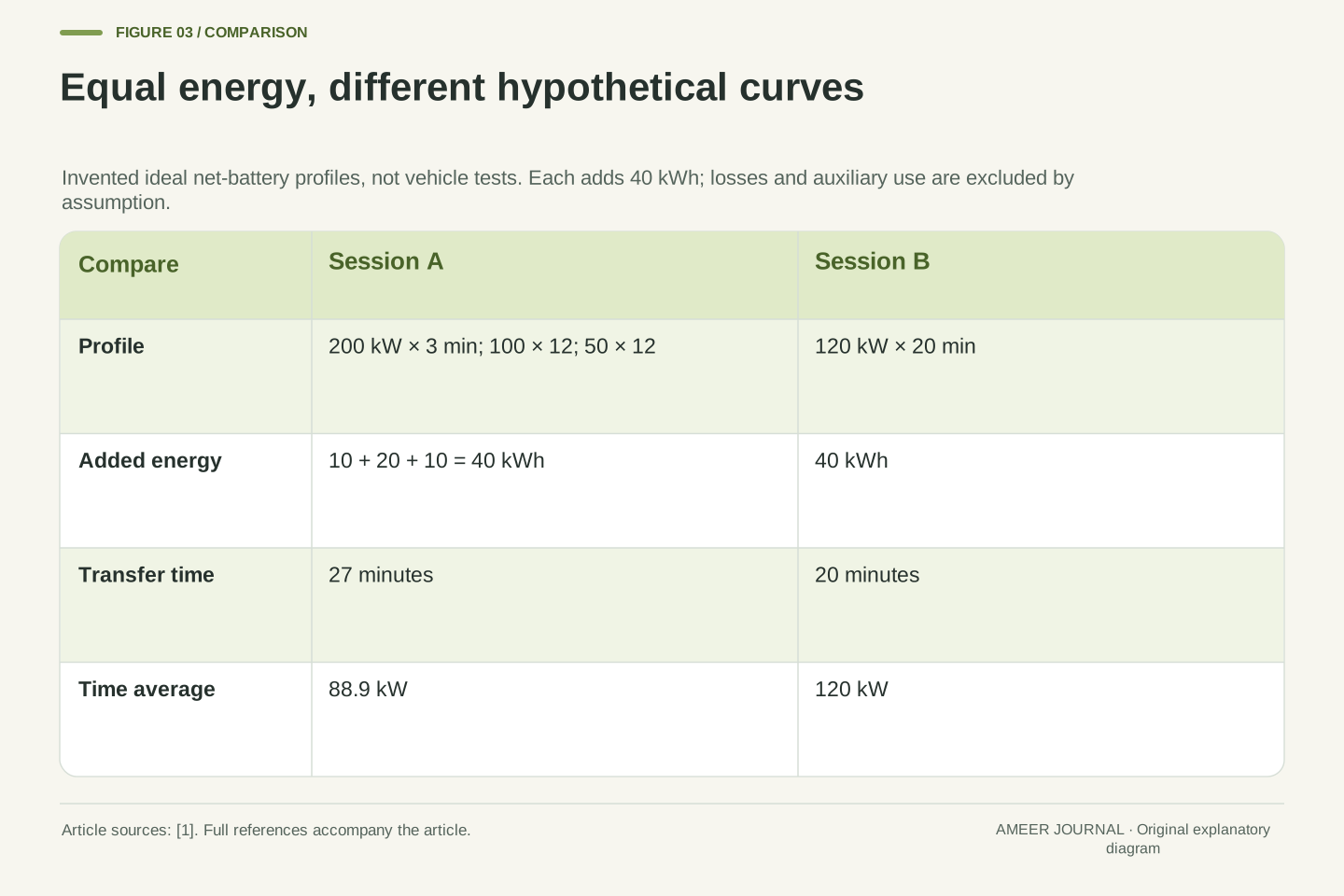
Consider two completely hypothetical sessions that each add 40 kWh. Session A starts at 200 kW for three minutes, then supplies 100 kW for twelve minutes, and finishes at 50 kW for another twelve minutes. The first part adds 10 kWh, the second 20 kWh and the last 10 kWh. The whole delivery takes 27 minutes. These are invented constant-power steps chosen so that every part can be checked by multiplication.
Session B supplies a steady 120 kW for twenty minutes. Twenty minutes is one third of an hour, so it also adds 40 kWh. It finishes seven minutes earlier despite having the lower peak. Nothing contradictory has happened: Session A's brief high rate did not compensate for its longer periods at lower power. The useful comparison is the same energy delivered over the complete interval.
Session A averages about 88.9 kW over its 27 minutes. Session B averages 120 kW over its twenty minutes. Do not turn that example into a claim that a particular low-rated station always wins. We deliberately specified both complete profiles. Without the profiles, session energy and elapsed time, a real peak-power advertisement does not provide enough information to reproduce this comparison.
Define hypothetical profile A by three piecewise-constant net battery-power segments: 200 kW for 3 minutes, 100 kW for 12 minutes and 50 kW for 12 minutes. Segment energy is P times minutes/60, giving 10, 20 and 10 kWh respectively. Total energy is therefore 40 kWh over 27 minutes. The early maximum is only one segment of the energy integral and receives no special weighting merely because it is the highest value.
Profile B holds 120 kW for 20 minutes. Its energy integral is 120 times 20/60 = 40 kWh. For this equal-energy comparison, B is seven minutes faster. A's time average is 40/(27/60) = 88.89 kW, while B's is 120 kW. Both averages are defined over their complete specified transfer intervals at the same idealized boundary. No percentage-to-energy conversion or vehicle-capacity estimate is required for this example.
The conclusion is conditional on the constructed profiles, not a general ordering by charger rating. Changing the requested energy window could change which parts of a profile are included and hence change the result. A useful comparison must disclose that window. A maximum quoted without duration cannot establish the integral, and a station capability quoted without the vehicle's accepted profile cannot establish the achieved session time.
Average power needs the whole clock
It is tempting to average Session A's three power numbers: 200, 100 and 50. That gives about 116.7 kW, but it is the wrong average for this session. The car spends only three minutes at 200 kW and twelve minutes at each lower rate. Giving every segment equal influence treats those unequal durations as though they were the same length.
Instead, add the energy from each segment and divide by the total time. That is how the previous section reached 88.9 kW. The same idea works when a session has many small changes. You need a reliable total energy reading and a clearly defined elapsed interval; you do not need to pretend the curve was flat. Compare readings from the same boundary so that the numerator and denominator describe one coherent event.
Decide how pauses are counted. In another invented example, 40 kWh transferred during twenty powered minutes averages 120 kW over powered time. If a five-minute interruption falls inside the elapsed charging interval, the same energy over twenty-five minutes averages 96 kW. Both calculations are correct for their stated clocks. A claim becomes confusing when it presents one clock while letting readers assume the other.
The arithmetic mean of A's segment rates is (200 + 100 + 50)/3 = 116.67 kW. That statistic weights segments equally; it does not weight time equally. The appropriate time average is (200 times 3 + 100 times 12 + 50 times 12)/(3 + 12 + 12) = 88.89 kW. The distinction is caused by unequal segment durations, not by any uncertainty in the constructed data.
For observations, calculate average power from total energy divided by a declared elapsed interval, or integrate a sufficiently resolved power series over that interval. An unweighted mean of readings is appropriate only when the sampling scheme gives them equal time weight. Irregular samples require duration weighting or a justified integration method. Preserve the start and end definitions so that someone else can reproduce the value rather than reverse-engineering an unexplained average.
State the treatment of zero-transfer periods. In a separate hypothetical event, 40 kWh over 20 powered minutes gives 120 kW, while including a 5-minute interruption gives 40/(25/60) = 96 kW. An active-transfer average and an elapsed-session average answer different operational questions. Neither should silently stand in for the other. Setup, payment and a queue can be reported separately when the reader's actual interest is total journey delay.
The same percentage window can hide different energy
Now consider two imaginary batteries with usable capacities of 60 and 90 kWh. For this example only, assume each percentage point represents a fixed share of that usable energy. Charging from 10% to 80% then adds 70% of capacity: 42 kWh to the smaller battery and 63 kWh to the larger one. The percentage labels match, but the energy amounts do not.
Suppose the smaller battery completes that interval in twenty minutes and the larger in twenty-five. The smaller one finishes its percentage window sooner. The larger one, however, adds 21 kWh more and averages 151.2 kW across its interval, compared with 126 kW for the smaller battery. Those statements can all be true at once. You must say whether you are comparing a percentage-window time or an energy delivery rate.
This arithmetic does not tell you which vehicle travels farther after charging. That needs a separate driving-energy assumption. Nor should the simple percentage mapping be treated as a precise measurement of a real battery's added energy. If a source supplies only percentage and nominal capacity, label the resulting energy estimate and its assumptions. An honest estimated comparison is more useful than a precise-looking number with an unexplained basis.
Let two hypothetical usable capacities be C1 = 60 kWh and C2 = 90 kWh. Assume fixed usable capacity and a linear mapping between displayed SOC and usable energy for this calculation only. A 10%–80% interval has delta-s = 0.70, yielding delta-E1 = 42 kWh and delta-E2 = 63 kWh. These are equal fractional windows, not equal-energy sessions. Real observations would need an independently justified energy mapping or a suitable energy measurement.
Assign constructed completion times T1 = 20 minutes and T2 = 25 minutes. The implied averages are 42/(20/60) = 126 kW and 63/(25/60) = 151.2 kW. Vehicle 1 has the shorter fractional-window time, while vehicle 2 has the higher average energy delivery rate and receives 50% more energy. There is no single winner until the evaluation criterion is stated. Neither metric alone supplies distance gained per minute.
An energy-per-distance value would be required to extend this comparison to added driving range. It must match the intended operating assumptions rather than being borrowed from an incompatible test boundary. Keep measured charger energy, estimated battery energy and percentage change in distinct fields. If the evidence only supports an estimate, round accordingly and show the capacity assumption instead of presenting derived decimal places as direct measurements.
Conditions can move the whole curve
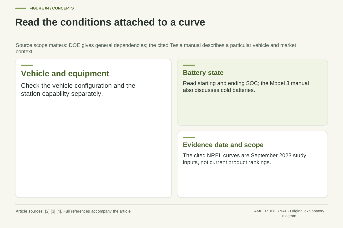
A charging profile belongs to a vehicle, a station and a set of conditions. DOE's charging guidance identifies battery state, capacity and type, vehicle charging capability, equipment and electrical supply among the factors affecting charging time. [3] A comparison that names only the station's largest printed number leaves out information needed to understand the result.
A manufacturer example makes the scope clearer. Tesla's U.S. Model 3 manual says the battery's rate is reduced when it is cold or nearly full. It also describes Trip Planner warming where that feature is available. [4] Those statements concern that manual and vehicle context. They do not establish one temperature threshold, preparation time or taper point for every electric car. Use your own model's current instructions when preparing for a journey.
Treat a curve from a review as evidence about the session described, then read its conditions. Look for the exact vehicle version, starting and ending charge, temperature information and how preparation was handled. If one of those fields is absent, preserve the uncertainty. You can still learn from the curve, but you cannot fairly assume that another car was measured under matching conditions simply because both charts use the same colours and axes.
The achieved profile is constrained by both vehicle acceptance and the available charging equipment. DOE lists battery SOC, capacity and type, internal charging capability, equipment power and electrical service among relevant charging-time factors. [3] A stationary nameplate rating is therefore a capability ceiling, not a complete time-varying transfer specification. Comparison records should distinguish the station rating from the observed or modeled profile actually used in the calculation.
For one explicitly scoped example, the U.S. Model 3 owner manual describes lower charging rates with a cold or nearly full battery and region-dependent Trip Planner battery warming. [4] This is manufacturer guidance for that context, not a cross-brand model of thermal behavior. The 2023 NREL profiles also vary by vehicle class and model year within the study's assumptions. [2] Neither source justifies assigning all cars one universal taper onset.
A fair empirical comparison would document configuration, software where known, SOC limits, relevant temperature and preparation information, charger capability and the measurement boundary. Missing conditions weaken comparability; they do not authorize an invented correction factor. Retain the original observation and mark what is unknown. If repeated sessions differ, investigate the changed conditions before averaging them into a single curve that appears more representative than the underlying evidence supports.
Choose an endpoint for the journey
A quoted 10%–80% time is a defined test window. It is not automatically the charge window you need for tomorrow's trip. If the next dependable stop requires more energy than that plan provides, the shorter quoted interval does not solve the journey. If you already have enough energy with an appropriate margin, waiting for an arbitrary percentage can add time without answering a practical need.
Battery-care instructions are another separate question. Tesla's cited manual qualifies its daily 80% advice to vehicles for which that daily limit is recommended; it is not written as a rule for every vehicle. The same manual warns about allowing its battery to reach zero. [4] Do not chase a low arrival percentage merely to reproduce a chart's impressive peak. Follow your vehicle's guidance and plan a suitable reserve.
For a planning worksheet, write the next leg's estimated energy need, the reserve you choose and the remaining energy already available. The added energy target is the gap between those values. Label it an estimate and revisit it when the route or conditions change. This approach makes the charging endpoint serve the trip. It also makes clear why a convenient comparison window and a sensible departure target need not be identical.
A standardized reporting interval and an operational departure constraint serve different purposes. A 10%–80% figure may facilitate comparison of a specified SOC window, but it does not establish sufficiency for the next leg or an optimal battery-care policy. Charging-time calculations should use the energy interval required by the planning problem. Substituting an attractive published interval can exclude the slower part that the actual itinerary still requires.
Keep manufacturer instructions scoped. The cited U.S. Model 3 manual qualifies its approximately 80% daily limit advice to vehicles carrying that recommended limit and warns about zero charge. [4] This does not justify generalizing a daily target across battery chemistries or vehicle configurations. A performance comparison is not an instruction to reduce the driver's reserve, alter battery safeguards or imitate a test's starting SOC in ordinary travel.
In a simple planning model, required addition is max(0, estimated next-leg energy + selected reserve − available usable energy). All three quantities must refer to compatible energy boundaries, and the target must fit within usable capacity. The expression is a bookkeeping relationship, not a range prediction. It becomes useful only when route estimates, access to the intended charging stop and uncertainty margins are assessed separately rather than hidden inside a nominal charging-time number.
Count detours and waiting as well as charging
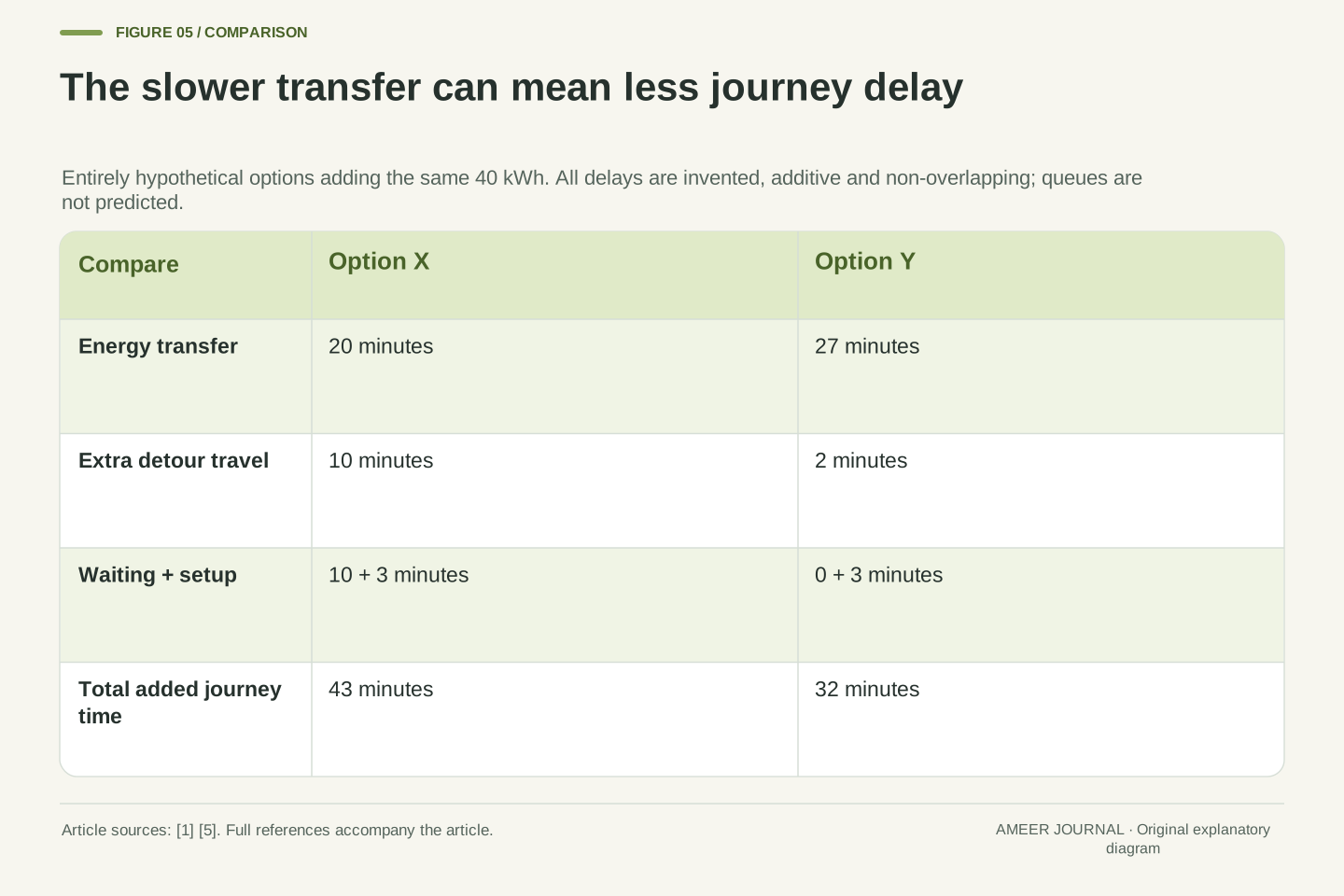
A faster energy transfer does not always make a faster journey. Consider two fictional route options that add the same 40 kWh at the same ideal boundary. Option X uses the twenty-minute session from our example, but adds ten minutes of detour travel, ten minutes waiting and three minutes of setup. The total added journey time is 43 minutes.
Option Y uses the slower, twenty-seven-minute session. Its detour adds two minutes, there is no wait in this invented scenario, and setup again takes three minutes. Its total is 32 minutes. Option Y therefore costs eleven fewer journey minutes even though it takes seven more minutes to deliver the energy. These figures are deliberately constructed, not reports of a station's reliability or an expected queue.
Count only extra time caused by the charging choice. Detour time means the difference from the otherwise relevant route, not the entire drive to the station. If lunch overlaps charging, do not count the overlapping minutes twice. Check connector compatibility and the intended stop using current vehicle information and route-planning resources; EPA specifically advises checking compatible connectors and adapters. [5] Then keep transfer time and total stop impact visible as separate results.
Extend the comparison boundary from energy transfer to incremental journey time. In a hypothetical additive model, option X comprises 20 minutes of transfer, 10 minutes of incremental detour travel, 10 minutes of queueing and 3 minutes of setup: 43 minutes total. Option Y comprises 27 + 2 + 0 + 3 = 32 minutes. Both add the same constructed 40 kWh, so the slower transfer option reduces modeled journey delay by 11 minutes.
The queue and route values are invented inputs, not inferred from either charging profile. NREL's cited infrastructure-sizing model expressly excludes queueing; it must not be cited as evidence for these delays. [2] Define the detour against a clear baseline route. The additive expression also assumes its components do not overlap. If a planned break and charging occur simultaneously, use an event timeline rather than adding both full durations and double-counting shared time.
Compatibility and access are prerequisites to the comparison, not minor adjustments to average power. EPA advises verifying the vehicle's connector and adapter compatibility and identifies route-planning resources for public charging. [5] Retain that check alongside any estimate of availability. Report charging duration, site occupancy and incremental journey delay separately when those intervals differ. This lets readers choose the result relevant to their trip instead of treating a laboratory-style transfer metric as a complete travel forecast.
Keep a session record you can interpret
A useful personal record begins before calculating an average. Write the date, vehicle, station, starting percentage, ending percentage and the reason for the stop. Record the beginning and end of the interval you want to compare. If the equipment provides an energy total, copy its label as well as its value so that you know what it claims to count.
Keep observations apart from estimates. A screen reading, a percentage-based estimate and a calculation from a published capacity are not interchangeable evidence. Note missing information plainly. A photo of a brief peak, for example, shows that moment; it does not establish the full session's average. Likewise, one successful session does not establish what every visit to that station will deliver.
Afterward, calculate energy divided by hours only when the energy figure and timing interval belong together. Add a short note about interruptions and preparation. If you compare two sessions, line up their endpoints and measurement choices before interpreting differences. The purpose of the record is to make your decision better, not to manufacture a ranking. A modest log with clear definitions can answer more than a dramatic peak number with its context removed.
Use a small record with explicit fields: timestamp, vehicle configuration, site and port, stated equipment capability, starting and ending SOC, energy value and its reported boundary, interval definition, elapsed duration and any interruption. Add preparation and environmental information when available. These are proposed recordkeeping fields, not a claim that every charger supplies each measurement or that consumer displays have laboratory accuracy.
Keep provenance attached to each field. Label a direct display reading, an estimate from SOC and assumed capacity, and a value from a published specification differently. Do not repair an incomplete record by fabricating missing temperatures, battery capacity or active-transfer time. A peak screenshot supplies a sampled power value at a moment; without additional data it cannot define the session integral or reveal how long that rate was sustained.
Compare only after aligning the reported boundaries and intervals. Calculate the average from compatible energy and duration, round to the input precision, and explain any excluded pauses. Repeated observations can reveal variability, but uncontrolled differences do not isolate a cause. Preserve the individual records when presenting a summary so that an unusual session or a changed starting SOC remains visible rather than disappearing into an unsupported single performance claim.
A practical check for the next charging claim
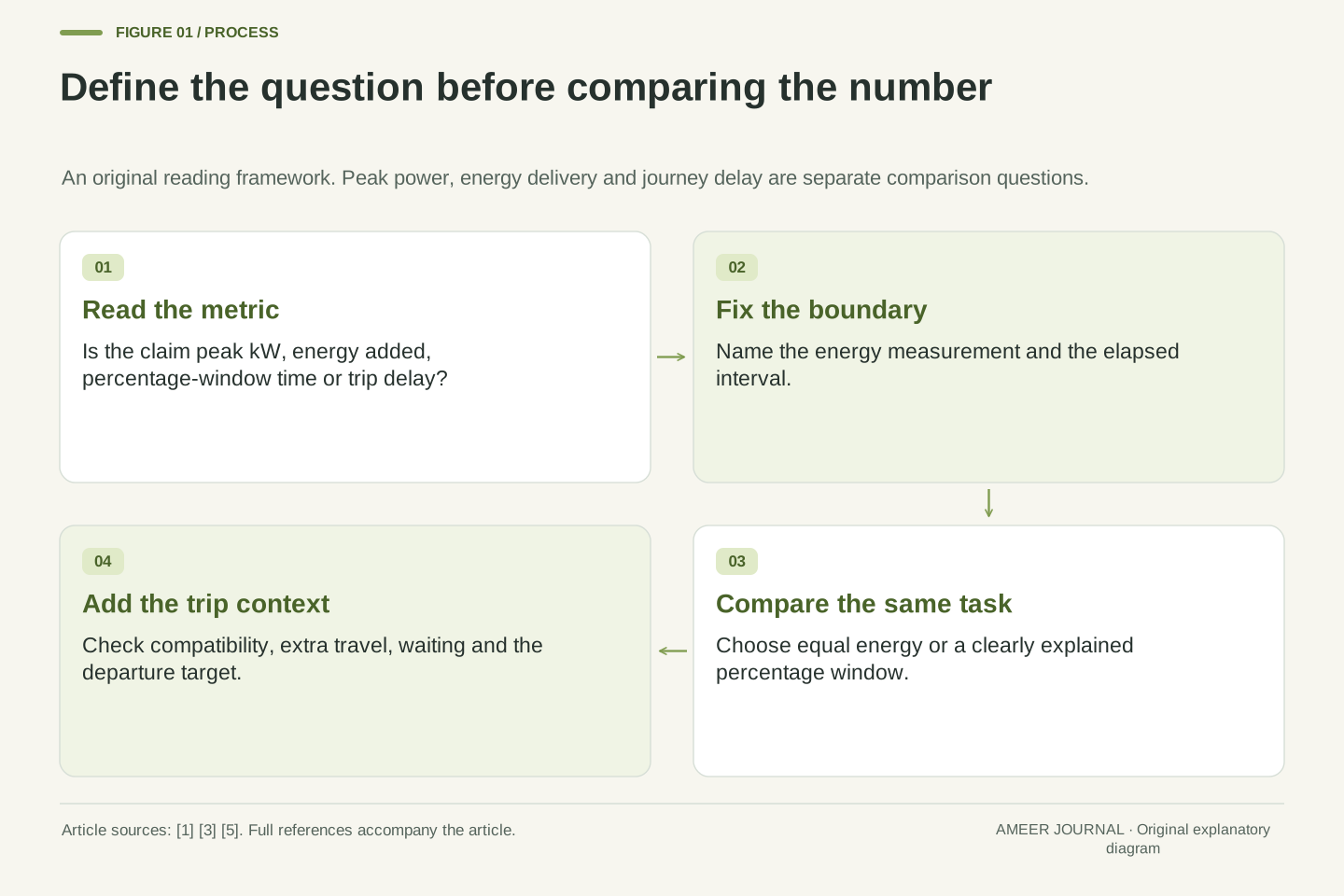
When you encounter a new charging claim, identify its question first. Is it the highest possible rate, time over a percentage window, time to add a fixed energy amount or the delay added to a journey? Write that answer in a sentence. If the advertisement does not make it clear, its big number is not yet a complete comparison.
Next, look for the exact vehicle and conditions, then read the axes and endpoints. Check whether an average uses the entire elapsed interval and whether the energy figure is measured or estimated. For two percentage-window times, compare the energy assumptions before calling one option faster. For a trip decision, include the relevant detour, likely access constraints and your required departure energy rather than borrowing the chart's endpoint without thought.
Finally, keep the result proportional to the evidence. Our invented 200 kW session lost an equal-energy comparison to a steady 120 kW session; our longer transfer then won a separate whole-journey example. Those results explain why the question and boundaries matter. They do not predict a named car's performance. A useful conclusion says what was compared, under which assumptions, and what remains unknown before you rely on it.
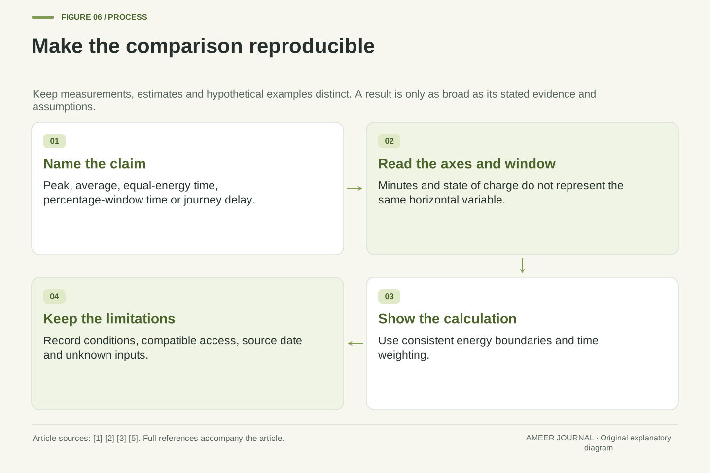
Evaluate a charging claim as a small reproducible calculation. First identify the dependent result: maximum power, transfer duration, energy-normalized average, fractional-window completion time or incremental journey delay. Then identify the independent conditions and the interval. If the claim does not define these, record the omission rather than choosing favorable assumptions on its behalf.
For a time-axis profile, integrate power over consistent units and boundaries. For an SOC-axis profile, justify the energy mapping before estimating duration. Use time weighting for averages, disclose pauses and avoid equating equal percentage changes with equal energy when capacities differ. For journey comparisons, add only the relevant non-overlapping delays. Confirm compatibility separately; a powerful but unsuitable connection is not an available charging option. [5]
End with a conclusion that can survive a change in one input. In the constructed 40 kWh comparison, 120 kW sustained for twenty minutes beats a 200 kW peak followed by lower rates. In the separate route calculation, a slower transfer wins because access delays differ. These conditional conclusions are the useful output. Keeping source dates, model scope, energy boundaries and hypothetical assumptions visible makes future updates possible without turning an old illustration into a false current benchmark.
Sources & further reading
Explore the references behind this guide. External pages may change after our review.
- Measuring electricity - U.S. Energy Information Administration (EIA)U.S. Energy Information Administration · Accessed 6 Nov 2026
- Fast Charging Infrastructure for Electrifying Road Trips to and from National Parks in the Western United StatesNational Renewable Energy Laboratory · Accessed 6 Nov 2026
- Alternative Fuels Data Center: Electric Vehicle Charging StationsU.S. Department of Energy / AFDC · Accessed 6 Nov 2026
- High Voltage Battery InformationTesla · Accessed 6 Nov 2026
- Plug-in Electric Vehicle Charging: The Details | US EPAU.S. Environmental Protection Agency · Accessed 6 Nov 2026
Article updated 6 Nov 2026.
Found something we should revisit?
Good explanations get better with thoughtful feedback.