What you’ll take away
- Relative airspeed determines aerodynamic force; vehicle ground speed enters ground-frame mechanical power.
- The familiar cubic power rule assumes still air, unchanged density and a fixed matched drag coefficient and area.
- Equal drag can give equal work per kilometre while different ground speeds give different power requirements.
- Compare drag coefficients with their reference areas and operating conditions, not as isolated rankings.
- Varying winds require the force/work calculation before averaging, and total battery consumption needs a wider model.
The air and the road provide different speed references
A car travelling into a headwind meets air faster than its speedometer reading alone suggests. That changes aerodynamic drag, the force associated with moving through the air. NASA identifies the relative velocity between an object and the air as the relevant speed for drag. [1][2] But another speed enters the power calculation: the car's movement relative to the road. Mixing those two references can produce a plausible-looking answer to the wrong question. The distinction matters when someone says that a headwind is equivalent to driving faster, or that a car's power demand must always follow a simple cube rule.
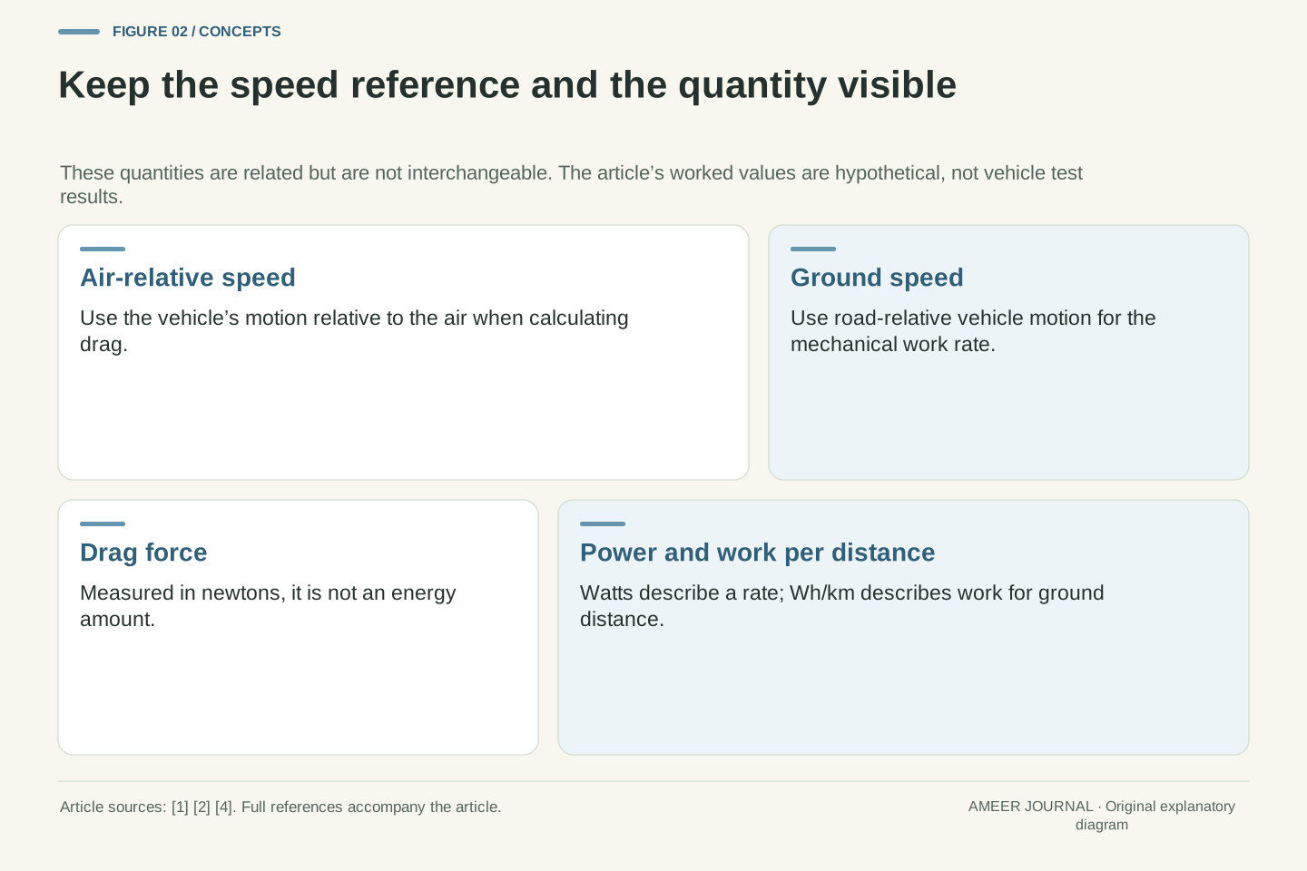
We will keep four quantities separate: air-relative speed, ground speed, drag force and vehicle-side mechanical power. We will also calculate energy per kilometre, which is different again from a power reading. The numerical examples are hypothetical, with fixed air density and drag area so one effect can be examined at a time. They are not test results, route predictions or suggested driving experiments. The aim is to read an aerodynamic claim correctly, then know what additional information would be needed before turning it into a battery-consumption or range claim.
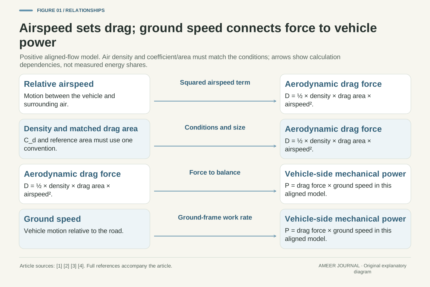
Aerodynamic force depends on motion relative to the surrounding fluid, while mechanical power transferred through a force must use velocity in the chosen energy-accounting frame. NASA explicitly identifies relative air velocity in its drag treatment. [1][2] The MathWorks longitudinal vehicle model separately calculates net relative airspeed for aerodynamic forces and multiplies drag force by vehicle longitudinal velocity for vehicle-side power accounting. [4] These are compatible statements. Confusion arises when the air-relative velocity used to calculate the force is silently substituted for the vehicle's ground-referenced velocity in a traction-power calculation.
This article uses a one-dimensional, steady-motion model on level ground, with drag opposing forward travel. It separates aerodynamic force, the mechanical power required to balance that force, and aerodynamic work per ground distance. Air density and a matched drag-coefficient/reference-area product are held constant in the numerical cases. Those restrictions exclude crosswind force resolution, changing body configuration, acceleration, grade, rolling losses, drivetrain conversion and auxiliary demand from the initial model. The examples are invented for dimensional and physical interpretation; none is a measured passenger-car coefficient, a driving recommendation or a complete prediction of battery energy.
Define the wind sign before adding speeds
For a straight headwind, think of the car and the air approaching each other. If the car moves at 20 metres per second (72 km/h) over the road and the air moves against it at 5 metres per second, their relative speed is 25 metres per second. In still air, the same car's relative airspeed would be 20. A tailwind of 5 would reduce it to 15 in this simplified straight-line case. The cited MathWorks vehicle model uses a headwind-positive convention for its wind inputs. [4] Other records can use different signs, so write the convention before inserting a wind number.
A sideways wind is not another number to add directly to the speedometer. It changes the direction of the incoming flow as well as its speed. NASA explains that the angle between a body and the flow affects drag. [2] Transport Canada's historical heavy-vehicle review also discusses the importance of this wind angle. [5] We will not borrow a truck's response as a car's response. Instead, the worked examples stay with headwinds and tailwinds directly along the travel line. A weather app's regional wind reading, without the direction and local conditions at the car, does not complete this calculation.
Choose v_g > 0 as the vehicle's ground speed and w_h as an along-road wind component defined positive for a headwind. Then v_air = v_g + w_h for the examples considered here. Thus v_g = 20 m/s with w_h = +5 m/s gives v_air = 25 m/s; w_h = −5 m/s gives 15 m/s. All of these air-relative velocities remain positive, so no force-direction reversal is involved. MathWorks documents this headwind-positive convention in the cited three-degree-of-freedom model. [4] It should not be assumed to match every simulator or meteorological data format without checking.
For oblique wind, relative velocity is a vector difference and the force relevant to longitudinal vehicle motion must be resolved consistently. The body's inclination to the flow can also change its aerodynamic coefficients. [2] The Transport Canada review makes that dependence explicit for heavy vehicles, especially at nonzero yaw. [5] Its truck-specific magnitudes and device results are not passenger-car data. A one-dimensional headwind model therefore cannot be extended to crosswinds simply by adding wind-speed magnitudes or retaining an unverified zero-yaw coefficient. We limit the arithmetic to aligned flow so the separate airspeed and ground-speed roles remain visible without hiding a directional model inside them.
Start with a complete still-air calculation
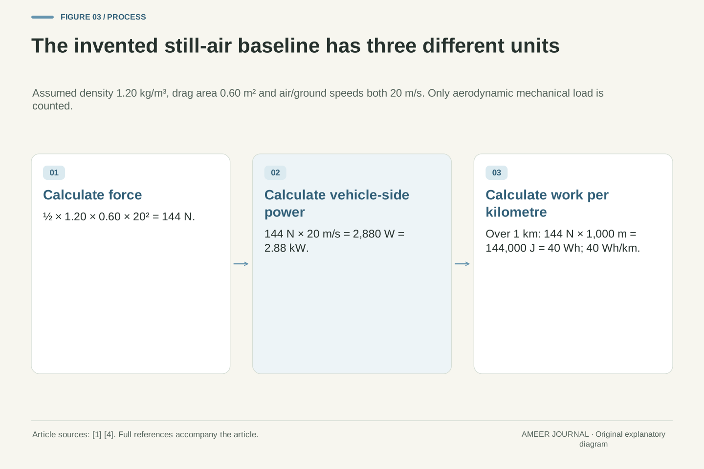
Set up an imaginary car with drag area 0.60 square metres and air density 1.20 kilograms per cubic metre. Drag area is the matched drag coefficient multiplied by its reference area; we will return to that pairing later. NASA's drag equation uses half the air density, multiplied by drag area and air-relative speed squared. [1] At 20 metres per second in still air, the calculation is ½ × 1.20 × 0.60 × 20² = 144 newtons. A newton measures force. This result is not yet a kilowatt number or an energy amount.
To balance that drag while moving over the road at 20 metres per second, the required aerodynamic mechanical power is 144 × 20 = 2,880 watts, or 2.88 kW. The force-times-vehicle-speed relationship appears explicitly in the vehicle model's power accounting. [4] Over one kilometre, work against this constant force is 144 × 1,000 = 144,000 joules. Dividing by 3,600 joules per watt-hour gives 40 Wh per kilometre. These are three descriptions of the same defined case: 144 N of force, 2.88 kW of power, and 40 Wh/km of vehicle-side aerodynamic work. None includes the other energy uses of a real car.
Use hypothetical ρ = 1.20 kg/m³ and C_dA = 0.60 m². With positive aligned relative flow, the NASA relation gives D = ½ρ(C_dA)v_air². [1] At v_air = v_g = 20 m/s, D = 0.5 × 1.20 × 0.60 × 400 = 144 N. The constant coefficient in front of v_air² is 0.36 in the corresponding SI combination. Dimensional checking gives kg/m³ × m² × m²/s² = kg·m/s², a force. Holding C_dA constant is an assumption for this comparison, not a declaration that a real vehicle has the same coefficient at every flow condition.
The ground-frame aerodynamic power requirement is P_aero = Dv_g = 2,880 W. MathWorks' drag-power expression uses force times vehicle longitudinal velocity consistently with this calculation. [4] At constant D, aerodynamic work over ground distance s is W_aero = Ds, so the work per kilometre is D × 1,000/3,600 = D/3.6 Wh/km = 40 Wh/km. Power divided by ground speed gives the same result after unit conversion. The distinction matters: force is in N, instantaneous mechanical power in W, and work per distance in Wh/km. Battery-terminal power would require a wider model than this isolated mechanical load.
Why the familiar cube rule has conditions
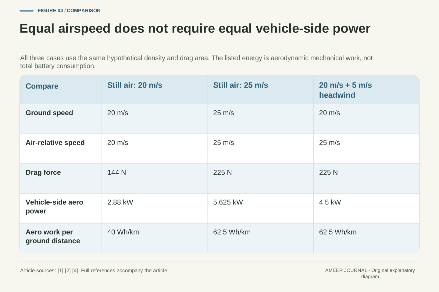
Now raise the imaginary car's ground speed from 20 to 25 metres per second while keeping the air still. Its air-relative speed also rises to 25. The same drag equation gives 225 N, and multiplying by ground speed gives 225 × 25 = 5,625 watts, or 5.625 kW. [1][4] The speed increase is 25%, but the drag increase is 56.25%. The aerodynamic power increase is about 95.3%. Those different percentages come from different questions: how strongly the air resists the car, and how quickly the car does work against that resistance.
In still air, with the same air density and drag area, force follows speed squared and mechanical power adds another factor of speed. That is the origin of the cube relationship. It does not say that every part of battery consumption follows a cube, nor that a wind change can be handled by cubing ground speed alone. Even in this invented faster case, aerodynamic work per kilometre is 225/3.6 = 62.5 Wh/km, which follows the force increase rather than the power increase. Power is higher partly because each kilometre is covered in less time. Keep that time distinction beside any speed-versus-consumption claim.
For v_g = v_air = 25 m/s in still air, D = 0.36 × 25² = 225 N and P_aero = 225 × 25 = 5,625 W. Relative to 20 m/s, the speed ratio is 1.25, the force ratio is 1.25² = 1.5625, and the power ratio is 1.25³ = 1.953125. These results follow from the stated drag equation and force-power relationship. [1][4] They correspond to 56.25% greater drag and 95.3125% greater mechanical aerodynamic power, under unchanged density and drag area. They do not establish the total propulsion or battery-power ratio of a production car.
The cubic rule requires the same velocity to appear in both roles: P_aero = ½ρ(C_dA)v_g³ only when still air makes v_air = v_g in this aligned model. For work per ground distance, W_aero/s = D, so the scaling remains quadratic under those assumptions. The 25 m/s case gives 62.5 Wh/km versus 40 Wh/km at 20 m/s. A claim about energy per kilometre therefore cannot be read as if it were a claim about instantaneous power. Conditions that change density, coefficient, direction or the relationship between airspeed and ground speed must be retained rather than compressed into a universal speed exponent.
A headwind changes the force without changing the road speed
Return the imaginary car to 20 metres per second over the road, then add the 5 metres-per-second headwind. Air-relative speed is now 25, so the drag force is again 225 N. The vehicle-side power is different from the faster still-air case: 225 × 20 = 4,500 watts, or 4.5 kW. [1][4] The car faces the same calculated drag force as the 25 metres-per-second still-air car, but it covers ground more slowly. That is the precise sense in which “equivalent airspeed” does not mean an identical mechanical-power requirement.
Using 25 in both places would produce 5.625 kW and silently answer a different question. For this car's work per road distance, the speed to multiply by force is its ground speed. Moving air has its own energy story; an air-relative description cannot simply replace the road-based vehicle calculation. [4] As a useful check, a body held stationary can feel an aerodynamic force while doing no forward mechanical work through ground motion. That does not mean the moving air has no energy or that a real parked vehicle uses no electricity. It only shows why a force and a vehicle-side power are different quantities.
Set v_g = 20 m/s and w_h = +5 m/s, giving v_air = 25 m/s. The same fixed-parameter drag model yields D = 225 N. However, the ground-frame power needed to balance this longitudinal force is Dv_g = 4,500 W, not Dv_air = 5,625 W. [1][4] The latter multiplication uses an air-relative velocity and cannot be substituted for the vehicle's tractive work rate in the ground frame. The wind participates in the wider energy balance; changing reference frames changes the force-power accounting without changing the physical aerodynamic force itself.
Relative to the original still-air 20 m/s case, the headwind raises both D and P_aero by a factor of 1.5625 because v_g remains fixed. In contrast, driving at 25 m/s through still air raised power by 1.953125. A stationary-body limit is another dimensional check: v_g = 0 makes the ground-frame force-work rate zero even when a headwind produces force. This observation is not a claim that wind energy vanishes or that auxiliary electrical consumption is zero. It isolates the mechanical term being calculated. Any total vehicle-energy model must keep those separate physical and electrical boundaries consistent.
Equal drag can mean equal work per kilometre and different power
Compare the two 225 N cases carefully. The faster still-air car travels at 25 metres per second and needs 5.625 kW for this load. The headwind car travels at 20 metres per second and needs 4.5 kW. Yet both require 225,000 joules of aerodynamic work per kilometre, or 62.5 Wh/km, because the force and the ground distance are the same. This result follows directly from force multiplied by distance, using the same constant-force assumptions as before. [1][4] A lower power reading therefore does not automatically mean lower energy use per kilometre.
Time explains the difference. One kilometre takes 40 seconds at 25 metres per second and 50 seconds at 20. Multiplying 5.625 kW by 40/3,600 hours gives 0.0625 kWh; multiplying 4.5 kW by 50/3,600 hours gives the same amount. That agreement is a check on the model, not evidence that the two real journeys would consume identical battery energy. Other loads can depend on time, temperature and operating conditions. The aerodynamic calculation has deliberately held them outside its boundary. It lets us compare this one load precisely without claiming to have solved the entire journey.
For a constant 225 N resistance, W_aero/s = 225 J/m = 62.5 Wh/km regardless of whether the force arose in our 25 m/s still-air case or 20 m/s plus headwind case. The ground-speed dependence cancels when P_aero = Dv_g is divided by v_g to obtain work per distance. [4] This cancellation assumes constant force and positive ground speed over the stated interval. It does not identify the source of the force as irrelevant; wind, density and coefficient still determine D before the distance normalization is performed.
The time integration confirms the result. At 25 m/s, a kilometre takes 40 s and 5.625 kW × 40/3,600 h = 0.0625 kWh. At 20 m/s, it takes 50 s and 4.5 kW × 50/3,600 h = 0.0625 kWh. These calculations distinguish instantaneous power, elapsed duration and work per distance without introducing a battery-efficiency assumption. A real comparison could still differ through propulsion conversion, rolling loads, climate control or thermal management. Thus equal isolated aerodynamic work is a bounded statement, not an equality between whole-vehicle energy totals or a recommendation about which driving situation to seek.
A lower drag coefficient needs its matching area
A drag coefficient is useful only with its reference-area convention. NASA explains that changing the chosen reference area changes the reported coefficient for the same measured drag; the pair must remain consistent. [1][3] For our car examples, drag area means the coefficient multiplied by frontal reference area. Imagine vehicle A with coefficient 0.24 and area 2.60 square metres. Their product is 0.624 square metres. Vehicle B has the higher coefficient 0.28 but the smaller area 2.10 square metres, giving 0.588 square metres. These are invented vehicles and numbers.
Under identical air conditions and the same aligned airspeed, vehicle A's drag would be about 6.1% higher because 0.624/0.588 is about 1.061. Its lower coefficient alone did not give the lower drag force. This comparison does not rank real cars or every aspect of their efficiency. It explains the missing size factor. When reading a coefficient, ask what area it uses and whether the other conditions match. A value normalized using one reference area cannot be compared blindly with a value using another, and a body-shape measure is not by itself a whole-vehicle energy measurement. [3]
C_d is dimensionless; A supplies the area scale in D = ½ρv_air²C_dA. NASA explains that the reference may be frontal, wetted or another stated area, with a compensating coefficient change when the convention changes. [1][3] The invariant product for a given measured force and flow condition is C_dA, provided the normalization is performed consistently. A hypothetical coefficient of 0.30 on a 2.0 m² reference and 0.20 on a 3.0 m² reference both represent C_dA = 0.60 m². The coefficient changed, but the physical drag described did not.
For two separate hypothetical vehicles using comparable frontal-area conventions, C_d,A = 0.24 and A_A = 2.60 m² give 0.624 m²; C_d,B = 0.28 and A_B = 2.10 m² give 0.588 m². Their force ratio at matched density and relative velocity is 0.624/0.588 = 1.061224. At the earlier 1.20 kg/m³ and 20 m/s, the forces would be 149.76 N and 141.12 N. This is a defined aerodynamic comparison, not a performance ranking. Different configurations, yaw angles or measurement conventions would require additional evidence before the same ratio could be applied.
A headwind and tailwind do not cancel after squaring
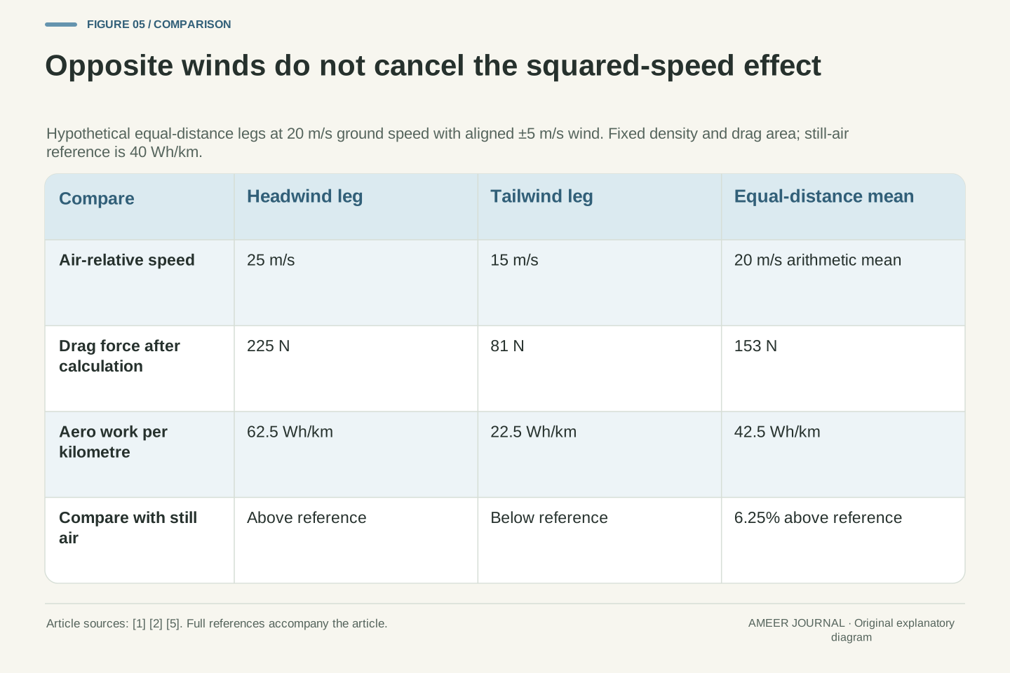
Consider two hypothetical equal-length parts of a journey, both at 20 metres per second over the ground. One has a direct headwind of 5 metres per second; the other has an equally strong direct tailwind. Keep all the earlier assumptions, including unchanged drag area and density. Air-relative speeds are 25 and 15. The drag forces are 225 N and 81 N. Their equal-distance average is 153 N, rather than the 144 N found in still air. The wind components average to zero, but the drag calculation squares relative speed before the results are averaged. [1][2]
The corresponding aerodynamic work values are 62.5 and 22.5 Wh/km, averaging 42.5 Wh/km. That is 6.25% above the still-air reference of 40 Wh/km. This is another invented model, not a rule predicting every return journey. Real winds can change direction and strength, routes can differ, and crosswinds can change the relevant coefficient. The historical Transport Canada review treats wind direction and wind-averaged drag as important in heavy-vehicle assessment. [5] Our simple arithmetic explains why replacing a varied wind history with one average wind number can lose information even before those extra complications are added.
For two equal-distance legs at fixed v_g = 20 m/s and w_h = ±5 m/s, the assumed relative speeds are 25 and 15 m/s. With ½ρC_dA = 0.36, their forces are 225 N and 81 N. The mean is 153 N. Algebraically, [(v_g + w)² + (v_g − w)²]/2 = v_g² + w², leaving a positive w² contribution relative to still air. [1][2] Because ground speed and leg length are equal, time weighting and distance weighting coincide in this particular example. They need not coincide for a general journey with different speeds or distances.
The work-per-distance mean is (62.5 + 22.5)/2 = 42.5 Wh/km, which is 1.0625 times the 40 Wh/km still-air reference. All conditions and coefficients were held fixed except the sign of the aligned wind. Do not apply 6.25% as a generic wind penalty. The Transport Canada review discusses wind-angle dependence and wind-averaged evaluation for heavy vehicles; its numerical results concern those vehicles and test conditions. [5] The general inference is narrower: nonlinear force response makes the distribution of relative flow conditions relevant. Averages should be formed after the appropriate force/work calculation, with the correct weighting for the quantity being reported.
Aerodynamic work is only one term in a vehicle model
An aerodynamic calculation does not contain the whole car. The vehicle must also handle other forces and loads, including changes in speed or height. The MathWorks body model includes mass, motion and road-grade terms alongside aerodynamic forces. [4] Transport Canada's heavy-vehicle review distinguishes aerodynamic resistance from rolling resistance and other contributions. [5] Those sources support keeping the terms separate; they do not supply one universal percentage of energy spent on drag for every EV. A car at steady speed on level ground is a simpler case than a journey with slopes, stops and changing thermal needs.
Time-dependent electrical demand can also distinguish two cases that had equal aerodynamic work per kilometre. For a separate invented example, a constant 1 kW auxiliary load running through the 50-second kilometre uses about 13.89 Wh. During the 40-second kilometre it uses about 11.11 Wh. Nothing about that calculation tells us which complete journey is better; all the other terms still need to be included. It simply shows why the earlier equality was deliberately limited to aerodynamic mechanical work. The correct next step is to widen the budget explicitly, not rename the 62.5 Wh/km drag result as measured battery consumption.
The vehicle longitudinal balance can include inertial, gravitational, aerodynamic and other force terms. The MathWorks documentation separates those contributions and provides their power accounting. [4] The Transport Canada review also treats aerodynamic and rolling resistance as distinct components of road load. [5] Its heavy-truck proportions and historical test procedures are not generalized to passenger EVs here. To move from isolated aerodynamic work to battery consumption, define drivetrain conversion and additional electrical demands, and integrate them over the actual operating history. A change in C_dA modifies one input to that wider problem; it does not directly establish an equal percentage change in total battery energy.
As a separate hypothetical electrical term, take a constant auxiliary demand of 1 kW. Its energy over the 50 s required for one kilometre at 20 m/s is 1 × 50/3,600 kWh = 13.8889 Wh. Over 40 s at 25 m/s it is 11.1111 Wh. This term is not added to the aerodynamic mechanical figures without also defining their conversion to the battery boundary. It demonstrates the distinct time dependence of another load and explains why equal aerodynamic work per distance does not imply equal total vehicle consumption. No optimum speed or real-world range is inferred from the incomplete model.
Read the quantity, the frame and the test conditions together
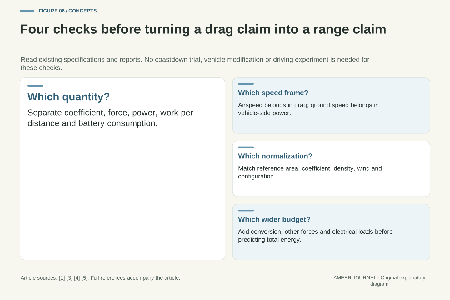
For the next aerodynamic claim, first identify the reported quantity: coefficient, force, power, work per kilometre or total battery use. Then ask for the matching area, air density, relative wind conditions and vehicle configuration. NASA's reference-area guidance makes the first pairing essential. [3] A historical Transport Canada discussion also shows why controlled tests and road conditions answer related but different questions. [5] We have used that report for physical and measurement context, not for a current technology ranking. A wind-tunnel result and a journey display should not be treated as interchangeable measurements simply because both mention efficiency.
You can apply this method to a specification or an existing report without changing the car or conducting a road test. For a headwind example, keep airspeed in the force equation and ground speed in vehicle-side power. For energy per distance, include the time or distance normalization explicitly. For a coefficient comparison, retain its area and conditions. Those checks explain the central result: driving faster and meeting faster-moving air can produce the same drag force while requiring different mechanical power. They also leave a clear boundary between an understandable aerodynamic model and the much larger task of predicting a real vehicle's journey energy.
A technically useful result identifies its observable, reference area, flow-relative velocity, vehicle-ground velocity, density, configuration and measurement method. NASA's area-normalization discussion and the historical heavy-vehicle review both show why coefficients and test conditions belong together. [3][5] Source type matters as well: NASA supplies physical relationships, MathWorks documents a vehicle model, and Transport Canada reports a heavy-vehicle literature review and testing context. None of the invented values in this article is re-labelled as an experimental passenger-car result. Historical test-method discussion is not a statement of the current legal certification procedure.
The compact calculation order is relative-flow state, matched aerodynamic coefficient and area, drag force, then ground-frame work rate or work per distance. Broaden to the battery boundary only after adding the necessary conversion and other-load terms. For oblique or varying wind, retain vector direction, coefficient dependence and appropriate averaging instead of using one scalar shortcut. These are report-reading and modeling checks, not instructions for coastdown trials or vehicle modifications. They make clear why a speed exponent, a small coefficient or a familiar power number can be correct within its definition while remaining insufficient to answer a different question about the whole car.
Sources & further reading
Explore the references behind this guide. External pages may change after our review.
- Drag Equation | Glenn Research Center | NASANASA Glenn Research Center · Accessed 6 Nov 2026
- Factors that Affect Drag | Glenn Research Center | NASANASA Glenn Research Center · Accessed 6 Nov 2026
- Size Effects on Drag | Glenn Research Center | NASANASA Glenn Research Center · Accessed 6 Nov 2026
- Vehicle Body 3DOF Longitudinal - 3DOF rigid vehicle body to calculate longitudinal, vertical, and pitch motion - SimulinkMathWorks · Accessed 6 Nov 2026
- Review of Aerodynamic Drag Reduction Devices for Heavy Trucks and BusesTransport Canada · Accessed 6 Nov 2026
Article updated 6 Nov 2026.
Found something we should revisit?
Good explanations get better with thoughtful feedback.