What you’ll take away
- Equal RMS voltage and total RMS current fix apparent power, but they do not by themselves fix real power.
- With pure sine voltage, an aligned current fundamental can coexist with a total power factor below 1 when higher current harmonics are present.
- The same total power factor can arise from different combinations of harmonic distortion and fundamental displacement.
- Power factor compares quantities at one AC boundary; conversion efficiency compares real powers across input and output boundaries.
- If voltage also contains harmonics, use the complete voltage-current relationship; the current-only THD factorization need not apply.
Two 10-amp records can describe different energy delivery
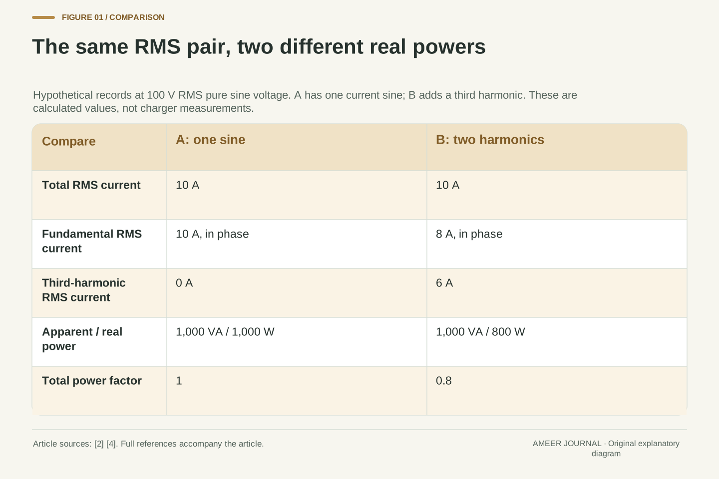
Imagine two invented AC input records. Both have an effective voltage of 100 volts and an effective current of 10 amps, yet one transfers energy at an average rate of 1,000 watts and the other at 800 watts. Even the second record's main current wave is perfectly aligned with the voltage. The missing piece is the shape of the complete current wave. Power factor compares average real power with the product of RMS voltage and RMS current; an aligned main wave alone does not determine that ratio when other current harmonics are present [2]. We will explain the unfamiliar terms and calculate exactly where the two answers come from.
This matters at the AC input of an electric car's onboard charger, which converts incoming AC electricity into DC electricity for charging the traction battery [1]. Texas Instruments' July 2017 engineering account describes a power factor correction stage, or PFC, before a further conversion stage; its ideal input-current objective is a sine wave aligned with a sinusoidal supply [3]. That is a dated engineering example, not a claim about every vehicle's design today. Our records below are hypothetical mathematical waveforms. They are not charger measurements, electrical settings or instructions for working on a circuit. The question is how to read the power quantities without confusing them.
Equal RMS voltage and RMS current fix apparent power S=V_rms I_rms, but they do not fix real power P, the mean instantaneous voltage-current product. Total power factor is PF=P/S [2][4]. An original single-phase example will hold voltage at a pure sine with V_rms=100 V and hold total I_rms=10 A. Different current functions then produce P=1,000 W or 800 W, even though the lower-power case has an in-phase current fundamental. This is a distinction between waveform magnitude, harmonic composition and correlation with voltage. It cannot be resolved by assigning one phase angle to the entire distorted current waveform.
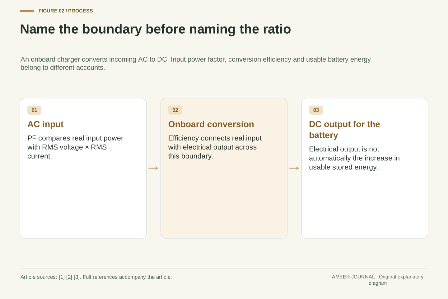
The relevant application boundary is the AC input of the onboard charger. AFDC describes the onboard unit's conversion of charge-port AC into DC for the traction battery [1]. TI's July 2017 account illustrates a PFC input stage followed by isolated DC/DC conversion and describes an ideal in-phase sinusoidal input current [3]. Neither the dated topology nor its product figures are universal present-day specifications. The calculations here use invented periodic functions, a common fundamental period and declared averaging boundaries. No vehicle, converter or instrument was tested, and no circuit implementation is proposed. DC electrical output will remain distinct from an increase in usable stored battery energy.
RMS keeps magnitude; real power also keeps timing
RMS stands for root mean square. For a changing current, square its values, average those squares over the chosen interval, then take the square root. Voltage is treated in the same way [4]. Squaring means that positive and negative parts do not simply cancel. RMS therefore gives a useful magnitude, but it does not preserve every detail of when the current is large or small. Two differently shaped waves can share that magnitude. A plain average of an alternating current can be zero while its RMS value is substantial, so those two kinds of average must not be exchanged.
Real power asks a different question: at each moment, multiply the voltage by the current, then average those products over a complete repeating cycle [4]. Here we call that result P and measure it in watts. Multiplying the separate RMS magnitudes instead gives apparent power, S, in volt-amperes, written VA [2]. Our two records both have S=100×10=1,000 VA. That statement contains no answer yet about whether P is 1,000 W, 800 W or another value. The same two magnitude summaries can conceal different joint patterns. We need the waves, or equivalent supported power information, to finish the calculation.
Let the averaging brackets mean a mean over one complete fundamental period T. Define V_rms=√⟨v²⟩, I_rms=√⟨i²⟩ and P=⟨vi⟩. OpenStax gives the instantaneous product, complete-cycle integral and RMS definitions; its native equations preserve the square roots that a flattened text extraction can lose [4]. In our finite periodic examples, the same T is used for every quantity. RMS is a norm-like magnitude of each waveform separately, whereas real power depends on their joint product. In particular, ⟨vi⟩ is not generally ⟨v⟩⟨i⟩, and neither expression should be silently substituted for V_rms I_rms.
Write θ=2πt/T. For v(θ)=100√2 sin θ V, the cycle mean of sin²θ is 1/2, so V_rms²=20,000×1/2=10,000 V² and V_rms=100 V. The factor √2 converts the chosen RMS coefficient into a pure sine's peak coefficient; it is not a generic peak-to-RMS rule for every shape [4]. Every current in the initial comparison will have I_rms²=100 A². Consequently S=1,000 VA throughout that comparison. Determining P still requires the current function, and total PF follows only after that mean product is known. The definitions already show why a pair of RMS values leaves information missing.
Build two equal-magnitude currents from different components
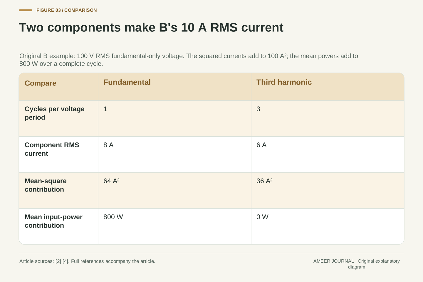
Record A uses one simple current sine wave. It repeats at the voltage's frequency, lines up with that voltage, and has an RMS current of 10 A. Record B combines two current waves. Its fundamental, meaning the part repeating at the voltage's frequency, has an RMS value of 8 A and lines up with the voltage. A second part has an RMS value of 6 A and repeats three times during each voltage cycle. This second part is the third harmonic. All these numbers and shapes are invented for the explanation. Harmonic current and displacement are separate ingredients in the power-factor relationship [2].
It would be wrong to add 8 A and 6 A and call B a 14 A RMS current. For these exact waves over a whole cycle, their mixed contribution to the mean square cancels. The squared RMS values add instead: 8²+6²=64+36=100 A². Taking the square root gives 10 A, matching A. This is an original calculation using the complete-cycle averaging method [4]. The two component waves still add at every instant, so B can have a large current at one moment and a smaller current at another. Equal RMS magnitude is compatible with those different distributions through the cycle.
Define record A by i_A(θ)=10√2 sin θ A and record B by i_B(θ)=√2(8 sin θ+6 sin 3θ) A. The coefficients 8 and 6 are RMS magnitudes of their individual sine components, not the peaks of the total current. The fundamental coefficient of B is positive and in phase with v. The 3θ term completes three periods while the voltage completes one. These are finite harmonic constructions rather than fitted or measured records. The distinction between current distortion and displacement is source-supported; the selected coefficients and all resulting numbers are our own [2].
Expanding the square gives i_B²=128 sin²θ+192 sin θ sin 3θ+72 sin²3θ in A². Over 0≤θ≤2π, each squared sine averages to 1/2 and the mixed-frequency product averages to zero. Thus ⟨i_B²⟩=64+0+36=100 A². A separately gives ⟨i_A²⟩=200×1/2=100 A². The mixed average can be derived directly from sin θ sin 3θ=(cos 2θ−cos 4θ)/2; each cosine integrates to zero over the stated interval. This extends the elementary cycle-average method illustrated in OpenStax [4]. It explains the quadrature addition here without claiming that arbitrary current components always add this way.
The third harmonic adds current without adding mean power here
Multiply A's current by the same voltage throughout the cycle and its average input power is 1,000 W. For B, the aligned 8 A fundamental contributes 100×8=800 W. The third-harmonic part contributes zero to the complete-cycle average of the voltage-current product. Its contribution is positive during some parts of the cycle and negative during others, with equal totals. This cancellation concerns that component's contribution, not a claim that B's whole input power must become negative. The averaging definition comes from the source; these two results follow from our explicitly chosen waves [4].
Two snapshots help expose the different timing. One twelfth of the way through the cycle, A's instantaneous power is 500 W while B's is 1,000 W. One quarter of the way through, A's is 2,000 W while B's is 400 W. These are momentary calculated values, not the cycle averages. B can exceed A at one point and still average less across the complete cycle. Nor has 200 W of incoming energy disappeared: B's average real input was 800 W from the outset. Its 1,000 VA label was never a separate 1,000 W delivery that must be split into output and waste.
For A, p_A=2,000 sin²θ W, hence P_A=1,000 W. For B, p_B=1,600 sin²θ+1,200 sin θ sin 3θ W. The first term averages to 800 W and the second to zero, yielding P_B=800 W. The same third-harmonic coefficient that contributed 36 A² to current mean square contributes zero mean power against this voltage because the voltage has no third harmonic. These are different products and different units. Whole-period orthogonality therefore reconciles the two results without any contradiction in energy accounting. The source supplies p=vi and cycle averaging; the harmonic extension is the displayed original derivation [4].
At θ=π/6, the exact instantaneous powers are p_A=500 W and p_B=1,000 W. At θ=π/2, they are p_A=2,000 W and p_B=400 W. A few samples alone do not establish the average; they illustrate why timing matters after the complete integrals have been evaluated. The component result ⟨v i_3⟩=0 also does not imply i_3=0, a zero instantaneous product, or a universal absence of hardware losses. No resistance or converter-loss model has yet been assigned. Subtracting P_B from S would mix two differently defined quantities and would not construct a dissipation term.
A well-aligned fundamental is only one of two factors
The displacement factor describes the alignment of the current's fundamental with the voltage in this sine-voltage model. It is 1 for B because those two component waves line up. The distortion factor asks what fraction of B's total RMS current belongs to that fundamental: 8÷10=0.8. Multiplying the two factors gives the total power factor, 1×0.8=0.8, agreeing with 800 W divided by 1,000 VA. TI distinguishes distortion and displacement in its power-factor expression [2]. It would be misleading to describe the whole distorted current as having one simple phase angle and use that angle alone.
Another way to express B's distortion is current total harmonic distortion, abbreviated THD. For this example, divide the RMS magnitude of all the higher harmonics by the fundamental's RMS magnitude. There is just one higher harmonic, so THD=6÷8=0.75, or 75%. That percentage is relative to the 8 A fundamental, not the 10 A total. The corresponding distortion factor is 1 divided by the square root of 1+0.75², which equals 0.8. We are using a pure sine voltage, a nonzero current fundamental and no constant DC current component. Those conditions make the factorization meaningful; they should travel with the result [2][4].
For the stipulated pure fundamental voltage, let I_1 be fundamental current RMS and φ_1 its displacement from voltage. Orthogonality gives P=V_rms I_1 cos φ_1. Dividing by S yields PF=(I_1/I_rms)cos φ_1. The first factor is the distortion factor in this setting; the second is fundamental displacement factor. For B, I_1=8 A, I_rms=10 A and cos φ_1=1, so PF=0.8. TI's native equation 2 presents the related THD expression, while the sinusoidal mean-power relation is explicit in OpenStax [2][4]. Our derivation states the voltage and averaging assumptions rather than applying the expression indiscriminately.
With finite integer harmonics, no DC term and I_1>0, define THD_I=√(Σ I_h²)/I_1 for harmonics h≥2. The squared-current sum gives I_rms²=I_1²(1+THD_I²), so PF=cos φ_1/√(1+THD_I²). B has THD_I=6/8=3/4 and distortion factor 4/5. The denominator convention matters: 6/10 would be a different ratio. A zero fundamental would make this THD definition undefined, and a voltage containing harmonics would change the mean-power calculation. A single total PF also cannot reveal which factor caused it. These are boundaries of the defined calculation, not evidence about any particular charger's spectrum.
The same power factor can hide two different current shapes
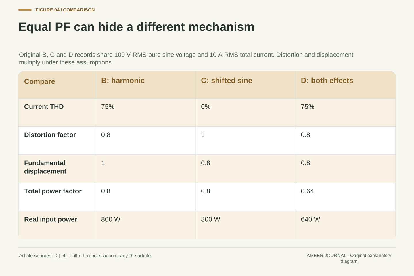
Now introduce record C. It is a pure 10 A RMS current sine wave at the voltage's frequency, but shifted in time. Choose its shift so that its displacement factor is 0.8. Because it contains no higher harmonic in this model, its distortion factor is 1. The total power factor is again 0.8, and its real input power is again 800 W. B and C therefore match in total current, apparent power, real power and total power factor. B reaches that result through its harmonic content; C reaches it through the phase displacement of a simple sine. A watt reading and a total power-factor reading cannot distinguish those two constructed explanations [2][4].
Record D combines both effects. Give its current fundamental an RMS magnitude of 8 A and a displacement factor of 0.8, then add the same 6 A third harmonic. The total RMS current remains 10 A, but the total power factor becomes 0.8×0.8=0.64. At 100 V RMS, real input power is consequently 640 W. Distortion and displacement factors are multiplied here, not added. The comparison also shows why an in-phase fundamental and a low-harmonic current are separate pieces of information. Neither statement alone establishes unity total power factor for every waveform; our four records identify the conditions behind each answer.
Set i_C(θ)=√2(8 sin θ−6 cos θ) A. This is a single fundamental sine with RMS magnitude √(8²+6²)=10 A, expressible as 10√2 sin(θ−φ_1), where cos φ_1=4/5 and sin φ_1=3/5. Thus THD_I=0, distortion factor=1, displacement factor=0.8, P_C=800 W and PF_C=0.8. By contrast, B has THD_I=0.75, distortion factor=0.8 and displacement factor=1. This is an original non-identifiability example: the same RMS pair, real power and total PF do not determine the harmonic decomposition or fundamental phase. It agrees with the sources' separate distortion and displacement mechanisms [2][4].
Define D by i_D(θ)=√2(6.4 sin θ−4.8 cos θ+6 sin 3θ) A. Its fundamental RMS is √(6.4²+4.8²)=8 A, and total RMS is √(8²+6²)=10 A. Fundamental displacement is 6.4/8=0.8, distortion factor is 8/10=0.8, and P_D=100×6.4=640 W. Therefore PF_D=0.64. The fundamental quadrature coefficient contributes to current mean square but not to real power against the sine voltage, just as the distinct-frequency term has zero mean product. This construction separates three orthogonal coefficient directions. It is not a claim that a specific PFC circuit produces D or that the coefficients can be adjusted independently in real hardware.
Matching real power changes the required current
So far we held total current equal and compared the resulting power. We can ask the reverse question: what happens if B's entire current wave is scaled until its real input power matches A's 1,000 W? Multiplying B by 1,000÷800=1.25 does that. The 8 A fundamental becomes 10 A, the 6 A third harmonic becomes 7.5 A, and the total RMS current becomes 12.5 A. The shape ratios stay the same, so the power factor stays at 0.8. This is a new comparison condition: equal real power now requires unequal current for these two waveform families.
Suppose the mathematical exercise separately imposes a 10 A RMS ceiling. A can deliver 1,000 W within that invented constraint, while an unchanged B-shaped waveform delivers at most 800 W at the same ceiling. Scaling B to 1,000 W would fall outside the permitted model. This follows from the definition P=V_rms I_rms PF [2]; it is not a recommendation to raise a charging setting. A real current rating, supported operating state and waveform would require their own documentation. The useful distinction is between holding current constant and holding power constant. Statements about 'more current' need to say which of those comparisons they mean.
For a fixed voltage function and positive scalar k, scaling the current by k scales I_rms and P by k, while leaving PF, THD_I and fundamental displacement unchanged. Apply k=5/4 to B: i_B,scaled=√2(10 sin θ+7.5 sin 3θ) A. Its squared RMS is 100+56.25=156.25 A², so I_rms=12.5 A, S=1,250 VA and P=1,000 W. The total PF remains 1,000/1,250=0.8. These results follow independently from the mean-product and mean-square definitions [2][4], rather than by interpreting an apparent-power difference as lost real power.
Under a separately stipulated I_rms≤10 A constraint and fixed 100 V sine supply, family A reaches 1,000 W at the boundary; the same B shape reaches 800 W there. The scaled B record is outside that feasible set. This is conditional algebra, not a circuit rating, thermal assessment or guarantee about a charger's controller. If waveform shape, voltage or operating conditions change with load, the fixed-PF scaling premise may cease to apply. The comparison therefore retains the waveform family as an input. It demonstrates precisely why equal-current and equal-real-power comparisons answer different questions, without importing an unstated hardware model.
Power factor does not tell us the conversion loss
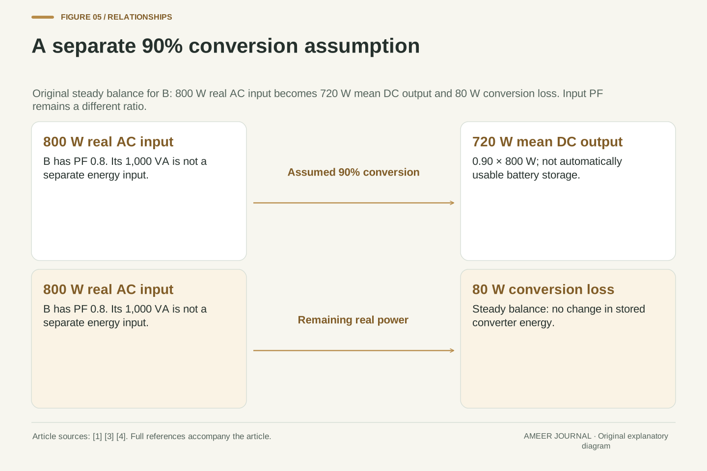
Return to the original B record: 100 V RMS, 10 A RMS, 1,000 VA apparent power and 800 W real input power. Now add a separate invented assumption: a converter delivers 90% of that real input power as mean DC electrical output. Its output is 0.90×800=720 W. If its stored energy is unchanged over the averaging interval, the remaining 80 W belongs in this model's conversion-loss account. The power factor of 0.8 did not supply the 90% assumption. The two ratios have different jobs: one describes the AC input waveforms, and the other connects real input with electrical output.
An onboard charger sits between the incoming AC and the DC supplied for traction-battery charging [1][3]. That physical boundary is why input power factor and conversion efficiency must stay separate. Calling the difference between 1,000 VA and 800 W '200 watts of heat' would invent a loss that the waveform calculation never established. Calling 720 W an increase in usable battery energy would skip another boundary as well. We have calculated mean DC electrical output, not battery chemistry or a vehicle's usable-energy display. A clearer record keeps the AC waveform quantities, converter output and any later storage account in separately named columns.
Introduce an independent conversion model with η=P_dc/P_ac=0.90 and P_ac=P_B=800 W. Here P_dc denotes mean DC electrical output, and the averaging interval is assumed to have no net change in stored converter energy. The stipulated balance gives P_dc=720 W and P_loss=P_ac−P_dc=80 W. None of these values is inferred from PF_B=0.8. The latter ratio uses P_ac and V_rms I_rms at the same AC boundary; η compares real powers across two boundaries. The onboard AC/DC role is documented, while the efficiency value and balance are explicitly hypothetical [1][3].
Apparent power S=1,000 VA is a product of RMS magnitudes, so S−P_ac is not an energy-conservation residual. Treating it as a watt loss would assign the wrong meaning to the operands. The mean DC output also does not establish the rate of increase of usable stored battery energy without a further storage and auxiliary-load model. The earlier vehicle-inverter and charging-schedule topics discuss their own energy boundaries; the new point here is that harmonic current can change total PF before any such conversion model is introduced. Preserving the boundaries prevents waveform distortion from being misreported as a measured conversion-efficiency loss.
Read the definitions before diagnosing a power difference
Consider a report that gives only '100 V, 10 A, displacement factor 1'. First establish that the voltage and current numbers are RMS values taken for the same input boundary and averaging interval. Next ask whether the voltage is being treated as a sine wave and whether 10 A means total current or just its fundamental. If 10 A is total current, both A and B fit the report, even though their real powers differ. The report therefore has too little information to establish 1,000 W. A total power-factor value or a properly defined real-power value would resolve that particular ambiguity in our model [2][4].
If the report instead gives total PF=0.8, that still does not identify the cause: B and C share that value. Look for separately defined current harmonic information and fundamental displacement when the question concerns waveform shape. If the question concerns converter loss, ask for real input and electrical output at named boundaries. These are questions about interpreting evidence, not a procedure for opening equipment or connecting test instruments. Preserve the source's model, date and operating conditions alongside the numbers. The remaining example changes just one assumption—voltage purity—to show why those conditions can change even a mathematically tidy answer.
A minimally interpretable record identifies the terminal boundary, averaging interval, RMS definitions, real and apparent power, and the waveform conditions under which any factorization is used. Suppose a report establishes V_rms=100 V for a pure sine, total I_rms=10 A and cos φ_1=1, but omits I_1 and harmonic content. A and B are two explicit solutions satisfying those givens with different P. The data are therefore insufficient for a unique real-power inference. This conclusion is established by constructive counterexample; it does not depend on an assumed instrument error or a claim about a real charger's performance [2][4].
Adding PF=0.8 determines P=800 W for that RMS pair, but still leaves the B-versus-C decomposition unresolved unless displacement or harmonic information is supplied. THD must specify its denominator, harmonic scope and current or voltage quantity. Conversion efficiency requires an additional input-output power boundary. These checks form an original interpretation method derived from the definitions and examples. They are not a metrology specification, compliance decision or hardware diagnostic. In particular, the current-only formula must not be carried into a record with distorted voltage merely because its current THD and fundamental phase are known. The next counterexample makes that limitation quantitative.
A voltage harmonic changes which current components transfer power
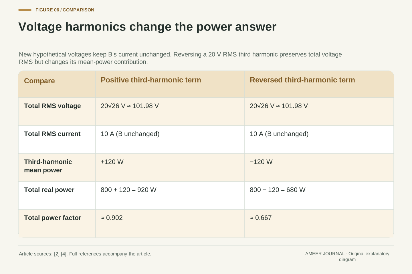
Keep B's current exactly as before, but replace the pure sine voltage with two new hypothetical voltage records. Both retain the 100 V RMS fundamental. Add a 20 V RMS third harmonic to one and reverse that harmonic's sign in the other. Both complete voltages have the same RMS value: the square root of 100²+20², about 101.98 V. Yet the third-harmonic voltage can now pair with the third-harmonic current. Its average-power contribution is +20×6=+120 W in the first record and −120 W in the second. The unchanged fundamental contributes 800 W, so the totals become 920 W and 680 W.
Both new records still have 10 A RMS current, the same current THD and an in-phase current fundamental. Their apparent power is about 1,019.8 VA, giving total power factors of about 0.902 and 0.667. The earlier current-only calculation would give 0.8, so it no longer answers this changed problem. These values come from averaging the full voltage-current products, using the same source definition and our newly stated waves [2][4]. The third-harmonic current did not acquire a different identity; the voltage now contains a matching component. Knowing which waveforms and boundaries a number describes is what makes the power record useful.
Retain i_B=√2(8 sin θ+6 sin 3θ) A and define v_±=√2(100 sin θ±20 sin 3θ) V. Both have V_rms²=100²+20²=10,400 V², so V_rms=20√26 V. Cross-frequency products still average to zero, but matching third-harmonic products no longer do. Direct integration of p=v_±i_B gives P_±=100×8±20×6=920 W or 680 W. This is an original extension of the complete-product definition [4], not an application of the earlier sine-voltage factorization. The sign reversal is a phase reversal of the voltage's third harmonic, leaving its RMS magnitude unchanged.
With I_rms=10 A, both apparent powers are S=200√26 VA. Consequently PF_+=23/(5√26)≈0.902 and PF_−=17/(5√26)≈0.667. Current THD remains 3/4 and fundamental displacement remains 1, yet 1/√(1+(3/4)²)=0.8 matches neither total PF. The definitions of RMS, real power and PF remain valid; the extra assumption required for the current-only decomposition has been removed [2][4]. Our bounded periodic counterexample does not describe every distorted supply or prescribe harmonic correction. It establishes a precise limit: the same current summary can support different power conclusions when the voltage spectrum and relative component phases are different.
Sources & further reading
Explore the references behind this guide. External pages may change after our review.
- How Do All-Electric Cars Work?U.S. Department of Energy Alternative Fuels Data Center · Accessed 7 Nov 2026
- How to improve the power factor of a PFC — SSZTDA4, September 2025Texas Instruments · Accessed 7 Nov 2026
- Are You On-board? Demystifying EV Charging Systems — SSZTA03, July 2017Texas Instruments · Accessed 7 Nov 2026
- University Physics Volume 2 — 15.4 Power in an AC CircuitOpenStax, Rice University · Accessed 7 Nov 2026
Article updated 7 Nov 2026.
Found something we should revisit?
Good explanations get better with thoughtful feedback.