What you’ll take away
- A short exposure at each row does not by itself make all rows capture the same moment.
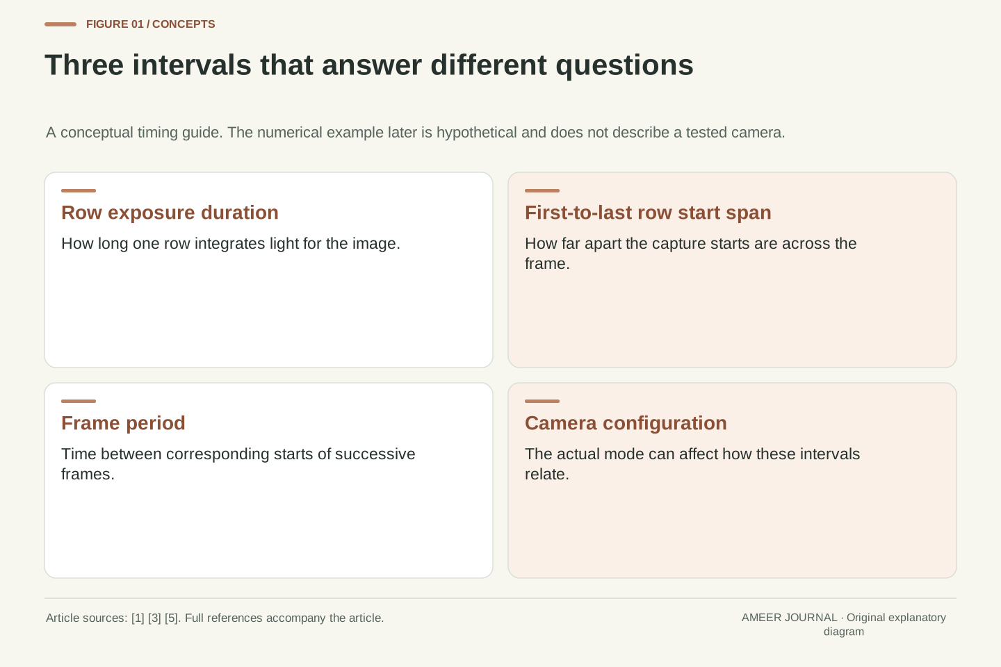
- Exposure duration, first-to-last row timing and frame period describe different intervals.
- Global exposure can be followed by sequential data readout without becoming rolling exposure.
- Scene motion and flickering light can produce different artifacts, so inspect shape and brightness separately.
- Use camera- and mode-specific evidence before inferring scan timing from frame rate, output size or a shutter label.
A sharp edge can still be in the wrong place
Imagine photographing a rectangular card as it slides sideways across a table. The printed edge looks crisp, yet the rectangle seems to lean. A short exposure may have stopped each small part of the image from smearing very far, while different parts were still recorded at different moments. Basler describes this timing offset in rolling-shutter cameras: rows begin exposing one after another, so rapid movement of the subject or camera can distort the assembled image [1]. The following card example is hypothetical; it is not a report from a camera test.
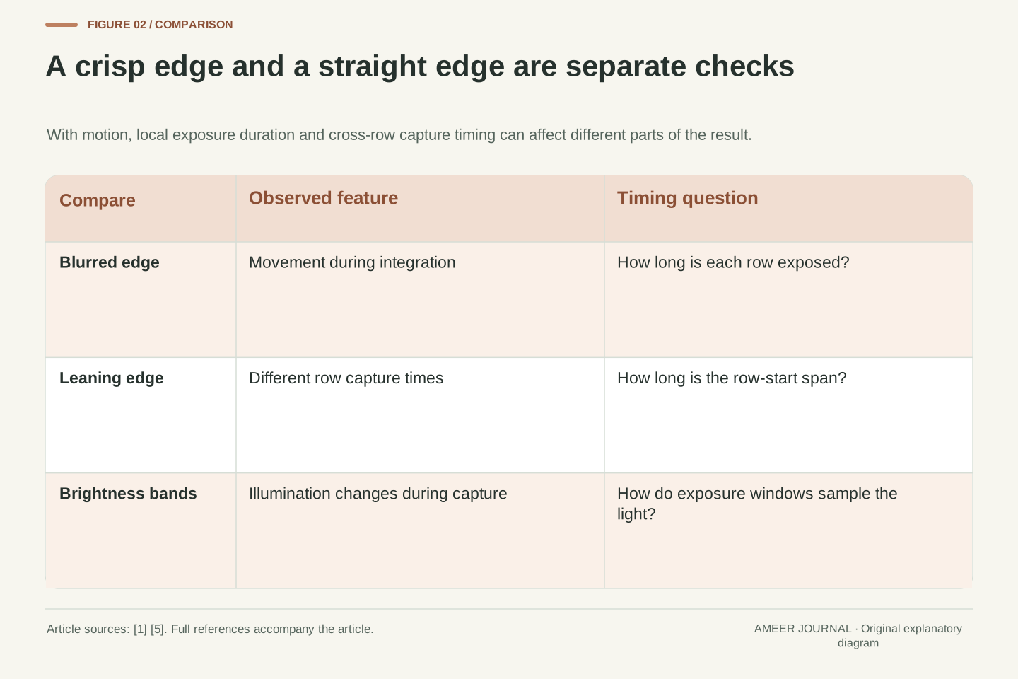
That distinction changes the question you ask. Instead of looking only for a faster shutter-speed setting, ask how much time separates the capture of the first and last parts of the frame. A camera can have a short exposure at each row and a much longer scan across the full image. We will follow an imaginary timing schedule, then use it to separate three problems: a blurred edge, a displaced edge and a brightness band caused by changing light. They can appear together, but the same adjustment will not necessarily improve all three [1][5].
Rolling-shutter geometry is a consequence of spatially varying acquisition time. A scene point's recorded position depends on when its sensor row is exposed; if the projected scene changes during the scan, rows do not share one temporal slice of the scene [1][2]. Short exposure duration limits motion within an individual row's integration window, but it need not eliminate the offset between those windows. Consequently, low local motion blur and visible geometric skew can coexist in a frame.
This article uses a uniform top-to-bottom row model to separate those effects. Row count, row-start interval, exposure duration and image-plane velocity will be explicitly chosen, rather than attributed to a product. The distinction is between integration time, cross-frame timing and the time between delivered frames. Basler's documentation supplies the basic sequential timing model, while Sony's flicker guide shows why changing illumination can make acquisition timing visible even in a stationary scene [1][5]. Actual readout architecture and mode-specific behavior still require camera-specific evidence.
Give the three clocks different names
Exposure time is how long a row gathers light for an image. The row-start gap is the short delay before the next row begins. A scan then carries that delay across many rows. The time between the start of the top row and the start of the bottom row can therefore be much larger than a single row's exposure. Basler documents equal exposure durations shifted from row to row, with the row interval varying by camera model [1]. Think of several people opening identical umbrellas one after another: equal opening durations do not mean simultaneous starts.
Frame rate is another number. It tells you how many frames are delivered in a second, not directly how the sensor timed every row inside each frame. For example, 25 evenly spaced frames per second means a 40-millisecond interval between frame starts. It does not, by itself, prove that the scan inside each frame lasts 40 milliseconds. That is a simple distinction between a repetition interval and the work inside it. Configuration can also matter: Basler documents a particular dart-camera design in which limiting interface throughput increases row readout time [3].
Define E as a row's exposure duration and Δ as the interval between successive row starts. In the simple uniform model, N rows create a first-to-last start offset of (N−1)Δ. Basler separately defines sensor readout time as NΔ, the sum of its row readout times [1]. These related intervals differ by one row interval. Use the definition attached to a manufacturer's timing parameter rather than treating every quantity called readout or scan time as identical.
The frame period is the interval between corresponding starts of successive frames. Its reciprocal is the frame rate in steady operation. It is a scheduling quantity, not enough information to reconstruct E or Δ. Real acquisition and transfer constraints can couple them, but the coupling depends on the architecture and mode. Basler's dart example explicitly ties row readout time to a throughput limit in a design without a frame buffer [3]. That is evidence of one such coupling, not proof that every consumer frame-rate setting changes row timing in the same way.
Follow the first row and then its neighbours
In our simplified camera, the first row starts at time zero. The second starts after one row-start gap, the third after two gaps, and so on. Each row remains exposed for the same duration, so its finishing time shifts along with its starting time. This is the sequence described in Basler's rolling-shutter explanation [1]. The rows do not necessarily wait for the previous row to finish gathering light. Their exposure windows can overlap, even though they begin at different moments.
Now imagine the card sliding steadily sideways. The upper rows see it a little earlier than the lower rows. When those rows are arranged in their normal positions to make the image, the card's edge may occupy a different horizontal position near the bottom. The stored rows have not been shuffled; the scene changed while they were being captured. The exact appearance depends on the motion and the scan direction [1]. A simple sideways translation can produce a lean in this model, while a different motion need not produce the same shape.
For row index r beginning at zero, assign an exposure interval from rΔ to rΔ + E. Adjacent windows overlap whenever E exceeds Δ, so sequential exposure start does not imply non-overlapping integration. This distinction matters when interpreting a timing diagram. Basler describes the same row-to-row shift at the beginning and end of exposure for its rolling-shutter sequence [1]. The simplified schedule here assumes uniform row timing and ignores sensor-specific reset, processing and blanking details.
If an image of a vertical edge translates horizontally at constant velocity, later rows encounter the edge at later horizontal positions. The result is a systematic row-dependent displacement in the assembled frame. This is a geometric model of scan distortion, not a claim that every artifact is a shear or that every camera scans in our chosen direction [1][2]. Rotational motion, changing velocity and a different acquisition order would require a different model. Keep the assumed image motion separate from a real object's speed in metres per second.
Work a hypothetical timeline in milliseconds
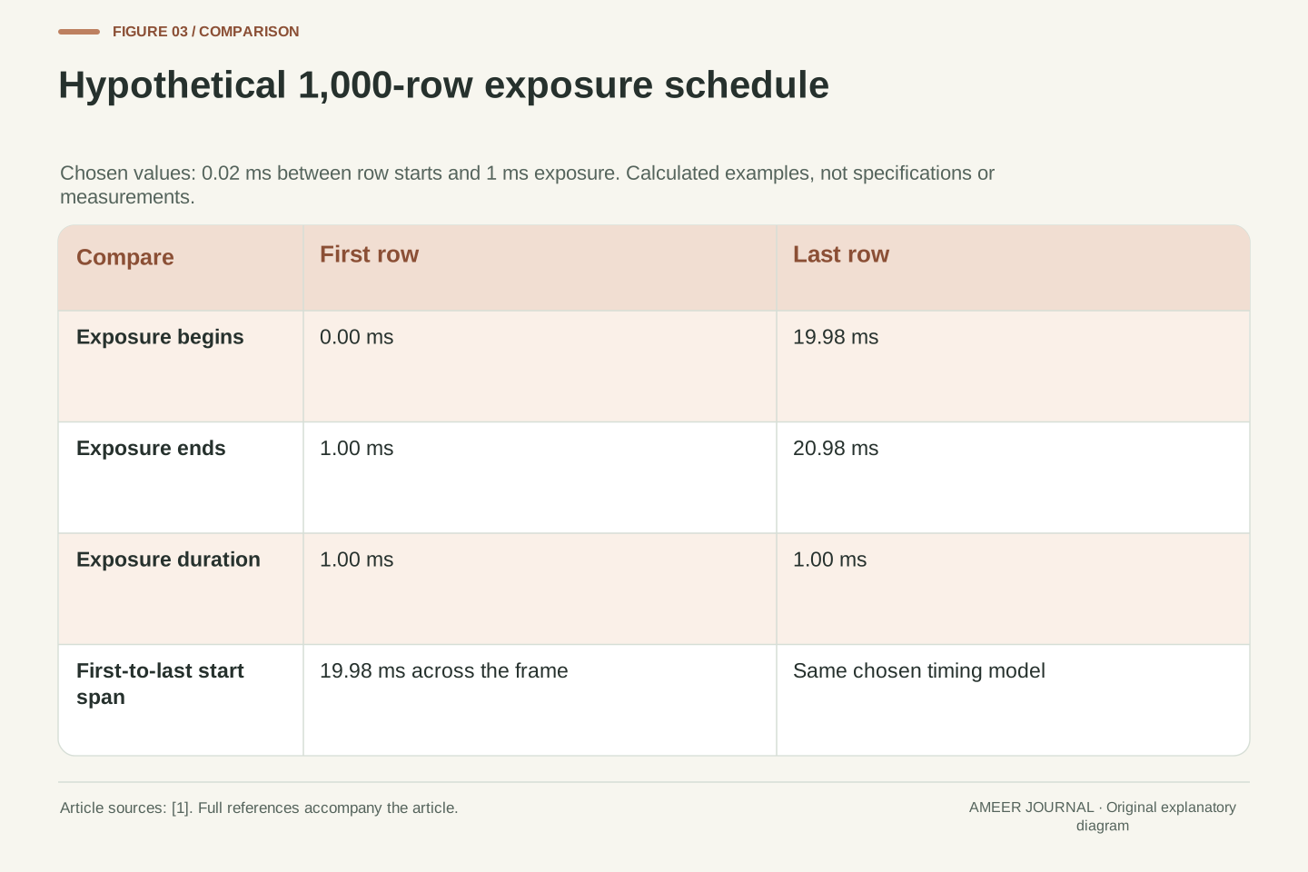
Choose an imaginary sensor with 1,000 rows. Let each new row start 0.02 milliseconds after the previous one, and let every row gather light for one millisecond. The first row is exposed from 0 to 1 millisecond. The last row starts after 999 gaps, at 19.98 milliseconds, and finishes at 20.98 milliseconds. Every row had a one-millisecond exposure, yet the top and bottom did not describe the same moment. These numbers are an original worked example based on the sequential timing rule, not specifications for a real camera [1].
There are two useful totals here. The gap between the first and last row starts is 19.98 milliseconds. Adding the one-millisecond exposure gives 20.98 milliseconds from the first start to the last finish. Basler's sum-of-row-readout-times definition would give 20 milliseconds for our chosen 1,000 rows and 0.02-millisecond interval [1]. The values are close but describe different endpoints. Keeping the labels attached prevents a rounded twenty-millisecond statement from being mistaken for either the exposure time or the complete duration during which any row is gathering light.
Set N = 1,000, Δ = 20 microseconds = 0.02 ms, and E = 1 ms. The first-to-last start offset is (1,000−1) × 0.02 = 19.98 ms. Row zero integrates over [0, 1] ms, and row 999 over [19.98, 20.98] ms. The union of all integration windows extends across 20.98 ms because these chosen windows overlap. This is a hypothetical uniform-timing calculation derived from the row sequence, with no asserted correspondence to a marketed camera [1].
Using Basler's NΔ readout-time convention gives 20.00 ms. Using first-to-last start time gives 19.98 ms. Using first start to last exposure end gives (N−1)Δ + E = 20.98 ms [1]. State the convention when comparing documentation or measurements; a small numerical difference need not indicate conflicting evidence if the endpoints differ. Furthermore, no frame rate follows uniquely from these values without a model for frame scheduling, overlap, blanking and transfer. The example describes one frame's timing, not a complete camera throughput specification.
Separate local blur from the change across rows
For a second part of the imaginary experiment, suppose the card's edge moves across the recorded image at 1,000 pixels per second. During a one-millisecond exposure it travels one pixel. Between the first and last row starts, it travels about twenty pixels. So an edge can be fairly crisp within each row while its position differs noticeably from the top of the image to the bottom. This calculation uses a deliberately chosen image speed and constant motion; it is not a measurement of how fast a person, car or camera must move [1].
Shorten the hypothetical row exposure to a quarter of a millisecond, while keeping the row timing unchanged. The travel during each exposure falls to a quarter of a pixel, but the first-to-last start gap stays 19.98 milliseconds. The model therefore predicts less local smearing without removing the cross-frame displacement. Real cameras may change other timing or exposure conditions when settings change, so check the actual mode. The lesson is to identify whether you are trying to reduce movement during each exposure or the time difference between rows.
Let the projected edge move at constant horizontal velocity v = 1,000 pixels/s. A simple box-integration model gives a motion extent vE = 1 pixel for E = 0.001 s. The difference between corresponding points in the first and last row windows is v(N−1)Δ = 19.98 pixels. Because all windows have equal duration and the assumed velocity is constant, comparing their temporal midpoints produces the same cross-row displacement. These are derived image-space quantities for the hypothetical sequence, not empirical camera performance [1].
Reduce E to 0.25 ms while retaining N, Δ and v. The integration motion extent becomes 0.25 pixel, but the row-to-row timestamp pattern is unchanged. A sharper-looking bent edge is therefore consistent with the model. This calculation deliberately holds scan timing fixed; a real exposure-mode change may alter more than E. It also ignores acceleration, optical blur, sampling and image processing. The purpose is to distinguish two causal intervals, not to predict an exact blur kernel or visible skew threshold for a particular photograph.
Global shutter aligns capture, even if data leaves later
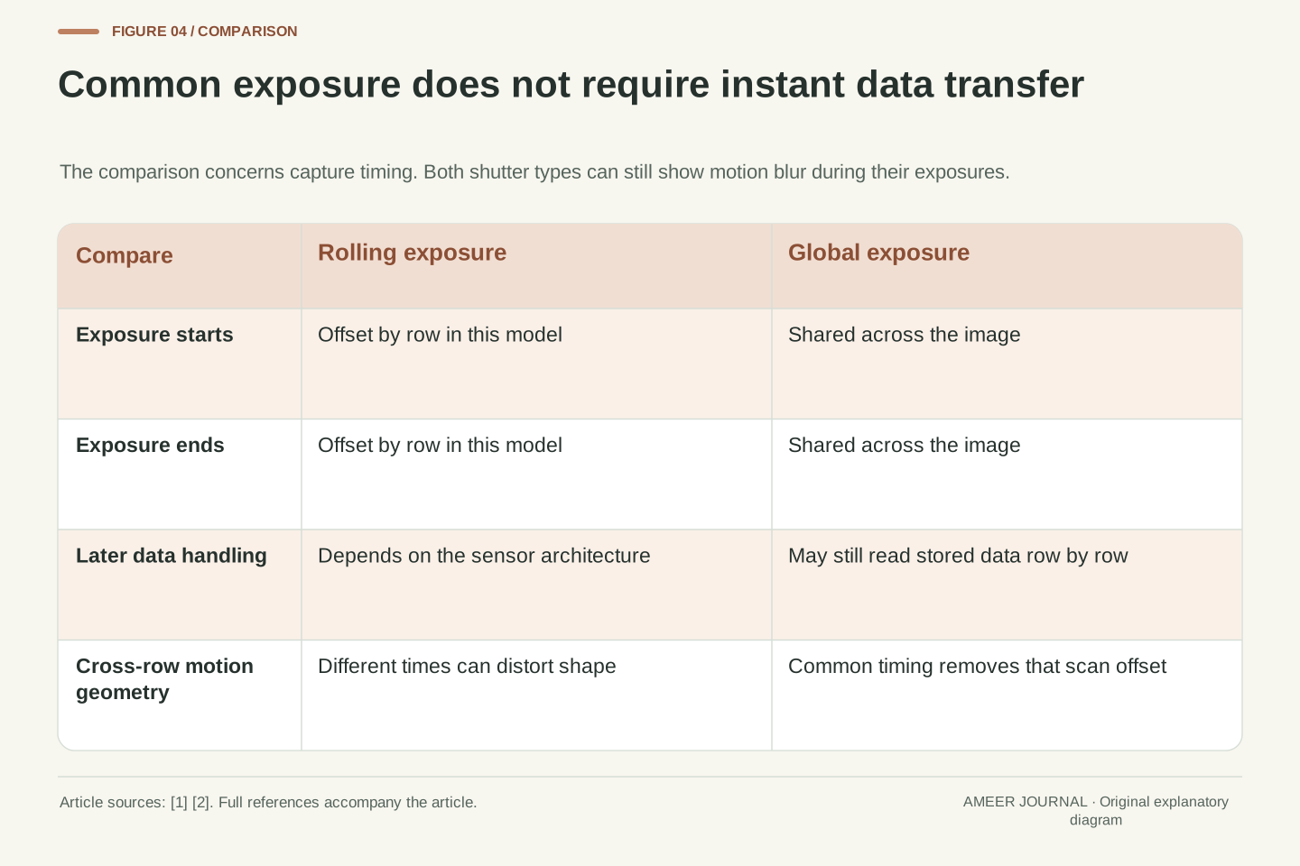
In a global-shutter capture, the pixels begin and end their exposure together. Basler explains that the saved pixel values can still be read out row by row afterwards [1]. Those later data transfers do not make the recorded scene a rolling-shutter exposure. The important distinction is when the light was captured, not whether every byte reached a processor at the same instant. Sony's description of its Pregius technology similarly separates whole-scene capture from subsequent processing [2].
A global shutter removes the row-by-row exposure-time difference responsible for the scan distortion in our example. It does not promise a perfectly sharp photograph. If the card moves during the common exposure interval, it can still blur; a lens can still be out of focus or have its own distortion. Read manufacturer phrases about distortion-free motion in that specific timing context [2]. The global-versus-rolling choice answers one question about capture timing. It does not replace decisions about exposure duration, optics, focus or the actual scene.
Global exposure requires a common integration interval across the image. Sequential downstream readout is compatible with that requirement if the captured information is retained for later transfer. Basler explicitly describes simultaneous exposure start and end followed by row-wise data readout, while Sony's Pregius explanation includes storage and subsequent signal processing [1][2]. Thus, describing a sensor as reading data line by line does not by itself establish rolling exposure. The timing of the scene integration must be identified.
For the same ideal translating edge, a global exposure assigns the same temporal window to every row. The scan-dependent displacement term vanishes, but the within-window motion extent vE remains. This follows from the same model used in the preceding calculation. Global capture consequently addresses temporal geometry, not every source of image degradation. Scope Sony's motion-distortion descriptions to the simultaneous-capture mechanism [2]; do not expand them into guarantees about optical distortion, motion blur, focus accuracy, image noise or the performance of an unspecified complete camera.
A timing number belongs to a mode, not just a body name
Even a useful readout number needs context. Basler's documentation says row intervals vary by camera model, and it describes how image-region height affects readout in its documented configurations. It also identifies models whose exposure still spans the full sensor despite a chosen image region [1]. That is why a simple rule such as smaller video frame equals faster scan is too broad. A saved image's size alone does not tell you which sensor rows were actually exposed or how the camera produced that file.
One concrete example comes from Basler's dart cameras. The company explains that limiting interface throughput can increase the time needed to read each row in that design [3]. This does not mean changing a consumer camera's recording bitrate produces the same effect. When looking up a timing measurement, keep the camera model, sensor mode, crop, resolution and relevant recording settings attached. If those details are missing, use the figure as incomplete evidence. A mode-specific demonstration is more useful than assuming every setting shares one advertised performance number.
Readout timing is a property of an acquisition configuration. Basler's documented NΔ relationship links row count and row timing, but the same page lists exceptions in which the first and last exposed rows remain the sensor's endpoints regardless of an image-region setting [1]. Therefore, output height is not a universally valid substitute for the number of rows participating in the acquisition sequence. Identify whether a reported crop changes sensor readout, subsequent processing or only file presentation.
The dart-camera note supplies a separate architectural example: a throughput limit can lengthen row timing because the described camera lacks a frame buffer [3]. Preserve that product scope. As a contrasting hypothetical, software could retain every second already captured frame, halving delivered frame rate without changing the timing inside any retained frame. This logical example shows why output cadence alone cannot identify sensor scan duration. Product documentation or a suitably described measurement must establish the relationship for the actual mode under discussion.
Changing light can create bands in a still scene
Movement is not the only change that rows can record at different times. Some artificial lighting varies in brightness or colour rapidly enough for different rows to receive different amounts of light. Sony's ILCE-9M2 flicker guide explains how these timing differences can appear as bands or partial colour changes [5]. The camera and card may both be still. Their shapes can remain straight while the lighting makes the capture timeline visible across the picture.
A universal shutter-speed recipe is not justified by that explanation. The lighting pattern, capture timing and available camera functions all matter. Sony's guide describes particular anti-flicker and variable-shutter features with model and firmware conditions; it is not a list of controls present on every current camera [5]. Check the guide for your own model and compare the recorded image, not just the live preview. That source specifically cautions that the preview and saved result may differ under some fast-shutter conditions. Record the light source and mode when investigating a banding problem.
For spatially uniform illumination with time-varying intensity L(t), a row's recorded illumination contribution depends on the integral of L over its exposure window. With rolling timing, those windows are shifted by rΔ. Even a static scene can therefore acquire a row-dependent brightness pattern. This is a mathematical restatement of the timing mechanism described in Sony's ILCE-9M2 flicker guide, not a new measurement of a lamp or a claim that all LED lighting has one modulation frequency [5].
Mitigation depends on the illumination waveform and the available acquisition controls. Sony's document distinguishes specific anti-flicker and fine shutter-adjustment capabilities, including model, shutter-type and firmware constraints [5]. Do not carry its historical mode restrictions or numerical timing examples across unrelated models. Nor should a banding pattern be attributed automatically to geometric rolling-shutter distortion: changing illumination and scene motion can coexist but require different checks. Compare actual saved frames under the intended lights, preserving the acquisition settings and the limitations of any preview-based observation.
Choose a control that changes the relevant interval
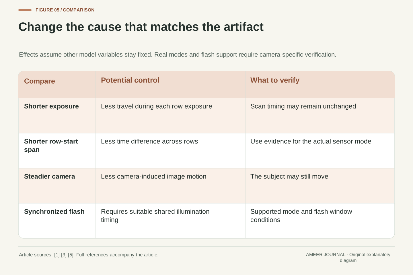
Holding the camera steady can reduce movement caused by the camera, but it cannot stop the card from moving. A shorter exposure can reduce travel during each row's capture, while a genuinely shorter scan can reduce the gap between early and late rows. These conclusions follow from the timing model, and the adjustments available depend on the camera [1]. Before changing equipment, identify which movement is in the image and which part of the timeline you can actually change.
Flash is also a timing problem, not an automatic cure. Basler describes synchronized flash arrangements for its industrial rolling-shutter cameras and a flash-window signal on supported models [1]. That is not a promise that an ordinary flash fired at any instant will illuminate every row evenly. In our one-millisecond-exposure example, the first row has finished long before the last row starts, so there is no instant when every row is simultaneously exposing. Use only the lighting synchronization and flash combinations documented for the actual camera; do not infer compatibility from the rolling-shutter label.
The model separates three interventions: reducing image-plane velocity v, reducing integration duration E, and reducing the start-time span (N−1)Δ. They act on different terms. Stabilizing camera position addresses only the component of image motion caused by camera movement; independent subject motion may remain. A mode change that genuinely shortens the row-start span reduces the cross-frame displacement for the same motion, while changing E alone does not [1]. The implementation must be verified rather than assumed from a menu label.
A synchronized flash can create a more nearly common effective illumination interval only under suitable acquisition and lighting conditions. In our simplified row schedule, the intersection of all integration windows has duration max(0, E−(N−1)Δ). It is zero for E = 1 ms and a 19.98 ms start span, so no single instant lies inside every row's integration interval. This is an original interval calculation. Basler's flash-window guidance is a documented industrial solution with its own operating conditions [1], not general authorization to apply arbitrary flash timing to every consumer camera.
Compare a simple scene and keep the original files
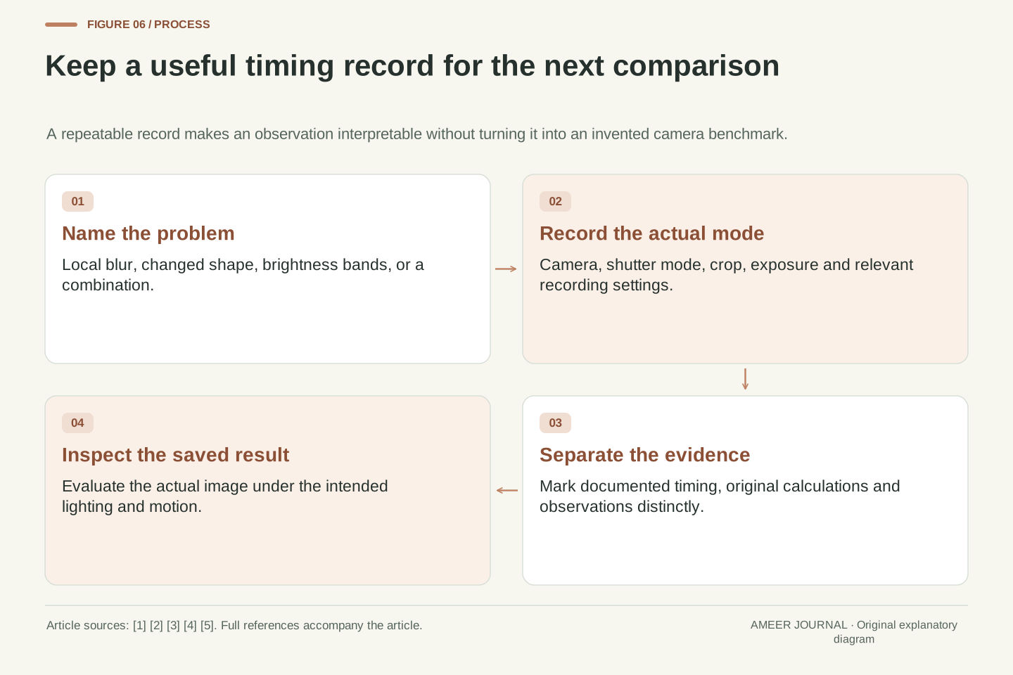
For a modest observation, use a printed card on a stable tabletop in comfortable, steady lighting. Make a stationary reference photograph, then compare it with a gently sliding card while keeping the camera steady. Keep the card flat so physical tilting does not become a competing explanation. Use ordinary handling rather than a fast spinning object or a moving vehicle. This is a proposed observation, not a test we performed, and the motion may be too slow for any scan distortion to be visible.
If your camera offers relevant shutter modes, consult its manual before changing them. Save the originals and note the mode, exposure time and lighting for each photograph. Ask separately whether the edge is blurred, whether its position changes from top to bottom, and whether brightness bands appear [1][5]. A visible difference can guide the next question, but this casual exercise cannot establish a precise readout time. The absence of an obvious lean does not prove global capture; the scene may simply not expose the timing difference clearly.
A useful observational record distinguishes a static reference from a controlled motion condition. A flat translated card is easier to reason about than an object rotating unpredictably in three dimensions. Preserve the same camera position and save original files, while documenting any changes to exposure, focus, shutter mode or illumination. This is a suggested qualitative exercise with acknowledged uncontrolled variables; it supplies no product measurements or claim of hands-on evaluation.
Inspect three outcomes separately: integration blur, systematic row-dependent edge displacement and spatial intensity variation. The first two relate to the motion model; the third can arise from the changing-light mechanism [1][5]. An observed skew is not enough to calculate Δ without a calibrated motion and projection model, and a visually clean image is not enough to identify the exposure architecture. Record what the files show, preserve the conditions, and avoid upgrading an informal comparison into a numeric camera specification or a universal assertion about a shutter technology.
Choose timing evidence before choosing a shutter label
For work involving motion, the useful questions are specific: how does this mode capture the frame, how long is its scan, and what happens under the lighting you intend to use? If a reliable timing value is unavailable, a carefully described demonstration of the actual mode may still be informative, but it should not be presented as a calibrated measurement. Keep exposure time and scan duration as separate entries in your notes. One very fast shutter-speed number cannot answer both questions [1][5].
Also avoid deciding every image-quality question from the shutter label. Sony describes noise-reduction and sensor-structure work in both its rolling-shutter and Pregius global-shutter technology pages [2][4]. Those descriptions do not establish a universal ranking of complete cameras. For the moving card, the important discovery was simpler: each row could be sharp while the frame combined different moments. Once you know which timing difference matters to your task, you can look for evidence about that difference and judge the actual photographs against a clear requirement.
A defensible comparison records exposure architecture, integration duration, scan-time definition, operating mode and illumination conditions. Verify whether a reported timing is first-to-last row exposure offset, a sensor readout parameter or an inference from an observed artifact [1]. Keep measured results separate from calculations and manufacturer examples. If a specification is missing, identify it as unknown rather than substituting reciprocal frame rate or the shortest advertised exposure setting.
Shutter architecture also does not fully specify image quality. Sony describes particular pixel, conversion and structural technologies in its rolling-shutter and Pregius families [2][4]. Those design descriptions are evidence about the named technologies, not a controlled ranking of every rolling and global product. In the hypothetical sequence, the distinction we could establish was exact: shorter E reduced integration travel, while unchanged Δ preserved the cross-frame timing difference. Carry that separation into the next camera comparison, and require mode-specific evidence for any broader performance claim.
Sources & further reading
Explore the references behind this guide. External pages may change after our review.
- Electronic Shutter Types | Basler Product DocumentationBasler · Accessed 6 Nov 2026
- Global Shutter Technology Pregius™ / Pregius S™ | Image Sensor for Industrial Use | Technology | Sony Semiconductor Solutions GroupSony Semiconductor Solutions · Accessed 6 Nov 2026
- Readout Time of Rolling Shutter dart Cameras Depends on the DeviceLinkThroughputLimit | Basler Product DocumentationBasler · Accessed 6 Nov 2026
- Rolling Shutter Technology | Image Sensor for Industrial Use | Technology | Sony Semiconductor Solutions GroupSony Semiconductor Solutions · Accessed 6 Nov 2026
- Understanding flicker | ILCE-9M2 Reducing issues from high-frequency flicker | SonySony · Accessed 6 Nov 2026
Article updated 6 Nov 2026.
Found something we should revisit?
Good explanations get better with thoughtful feedback.