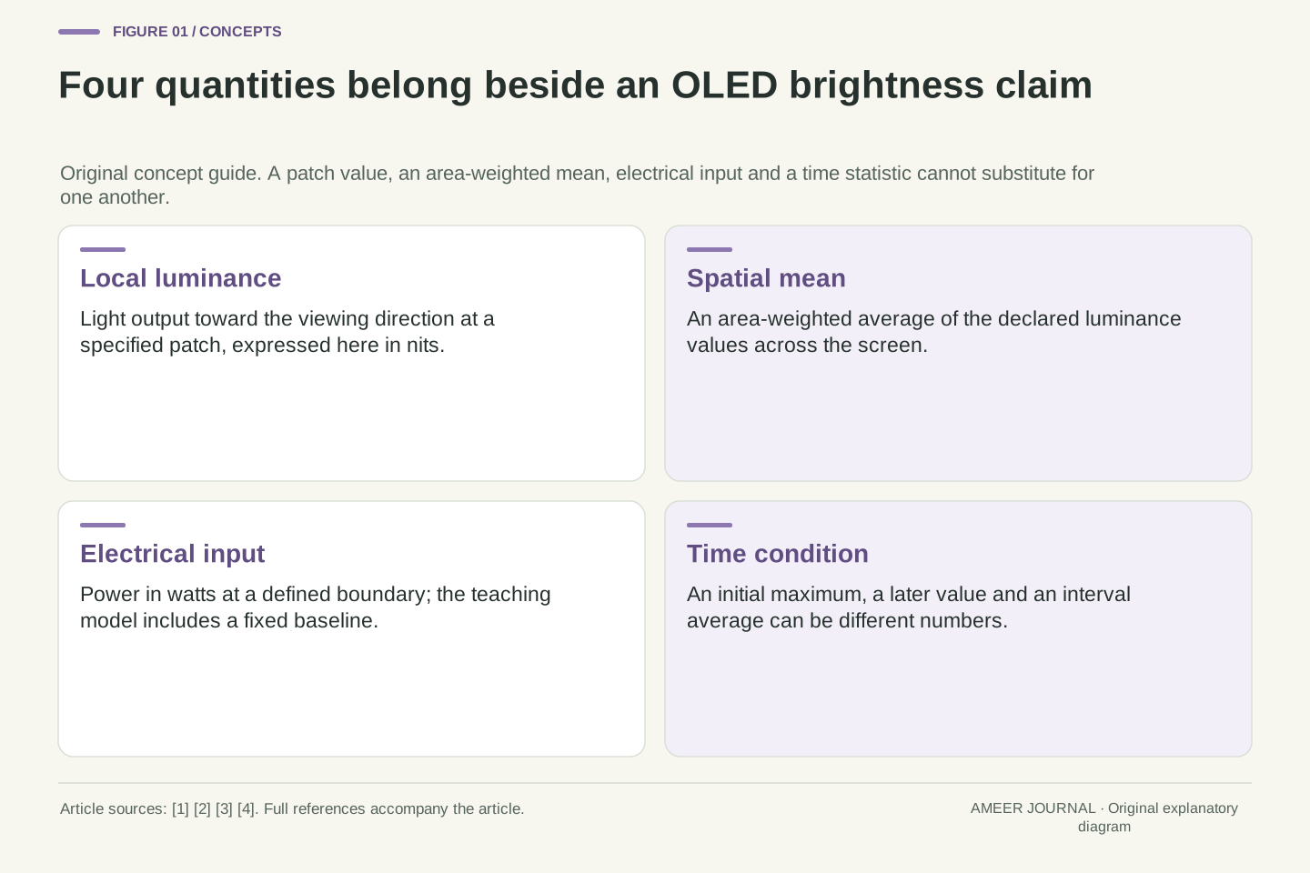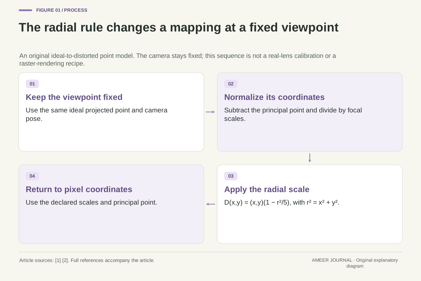
What you’ll take away
- Keep lens mapping, camera viewpoint and the chosen output geometry separate.
- A point can move toward the centre while an offset line bows outward relative to its endpoint chord.
- A centre-crossing line can stay straight under nonzero radial distortion, so that observation alone does not identify the coefficient.
- Correcting an observed point uses the inverse map; rendering an ideal output can use the forward map to find source samples.
- Coefficients need a model, normalization and domain; interpolation and output coverage are separate choices.
A curved edge and a changed viewpoint are different questions
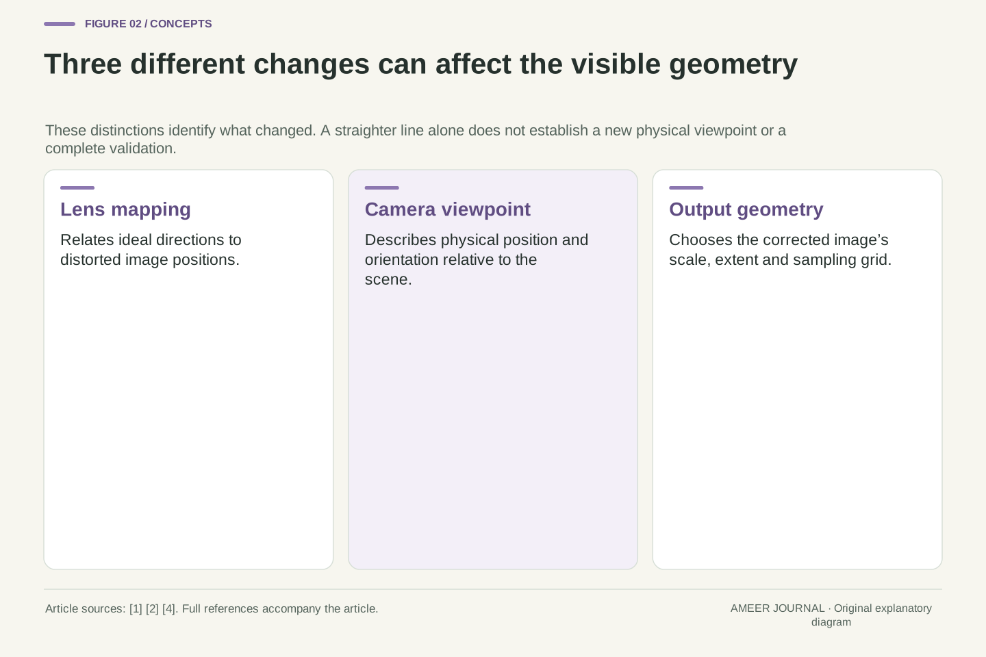
A doorframe looks bowed near the edge of a photograph. Applying lens correction makes it straighter, yet the camera has not moved and the scene has not been photographed again. The correction changes the mapping between image positions. Camera models distinguish that lens-distortion mapping from the camera's position and orientation in the scene. [1][2] Keeping those jobs separate helps explain why straightening a curve need not remove every effect of where the photograph was taken.
We will use an original radial model with a fixed camera and a few invented coordinates. Its coefficients, dimensions and sample values are teaching inputs, not measurements of a lens or results from image-editing software. The model will explain a surprising combination: individual points move toward the image's reference centre, while a line through those points bows outward. We will then distinguish correcting an observed point from filling the pixels of a corrected image. Those two operations follow the same relationship in different directions, which is why the word correction alone leaves important details unstated.
Separate camera pose, ideal projection and lens-distortion mapping. The first describes the camera's relation to the scene; the last changes where projected directions appear in the image. OpenCV's calibration model includes radial and tangential terms, while MathWorks explicitly separates extrinsic, intrinsic and distortion parameters. [1][2] Correcting a radial map at fixed pose therefore does not establish a new physical viewpoint, recover an occluded scene or validate a ground-distance calculation.
Our original fixture isolates a zero-skew, single-coefficient radial map with all tangential and higher-order terms zero. We keep pose fixed, declare the coordinate scale and restrict the map's domain. No camera, calibration solver or image library is executed. The worked consequences concern an offset line, a centre-crossing line, inversion and raster lookup. A separate scalar interpolation patch and a named fisheye-model comparison expose two additional boundaries: a coordinate map does not select a unique sampling rule, and coefficient labels do not identify a projection model.
Give the coordinates a centre and a scale
The radial calculation uses distances from a reference point called the principal point. It also uses a focal scale measured in pixels. MathWorks describes converting image coordinates into normalized coordinates by subtracting that point and dividing by the focal scale; the resulting numbers have no physical length unit. [2] This matters because inserting a raw pixel count into a formula written for normalized distances changes the meaning of the coefficient.
For our model, choose the principal point at pixel coordinates (800, 600) and use a focal scale of 1,000 pixels in both directions. An ideal point at (1,300, 600) is 500 pixels to the right, so its normalized coordinates are (0.5, 0). A point at (1,300, 1,100) becomes (0.5, 0.5). The reference extent is 1,600 by 1,200 in continuous image coordinates. These choices put the principal point at its centre for this example; that equality is an assumption of the fixture. The scale of 1,000 pixels is not a 1,000-millimetre lens.
Let ideal image coordinates be (u,v), principal point (c_x,c_y)=(800,600), and focal scales f_x=f_y=1,000 pixels, with zero skew. Normalize using x=(u−800)/1,000 and y=(v−600)/1,000. MathWorks identifies the principal-point and focal-scale pixel units and explicitly defines normalized coordinates as dimensionless. [2] The distortion polynomial below acts on these normalized coordinates, before conversion back to pixels. Our equal scales make the pixel-distance conversion particularly simple. If the two scales differed, the normalized radius would still use the two separately normalized components, not one unqualified distance measured in pixels.
Use a continuous reference extent [0,1600] × [0,1200]. Its corner offsets normalize to (±0.8,±0.6), whose radius is one. We will analyze the disk r≤1 containing that extent. The ideal point (1300,600) normalizes to (0.5,0), while (1300,1100) becomes (0.5,0.5). These are declared geometric coordinates, not a claim about a library's pixel-centre convention. Keeping normalization explicit prevents a coefficient defined for dimensionless radius from being reused against unscaled pixel distance or a different principal-point origin.
A radius-dependent scale moves points by different amounts
In the polynomial radial model documented by OpenCV, each coordinate is multiplied by a scale that depends on distance from the centre. [1] We choose a simple case: the scale is one minus one-fifth of the squared radius. Both coordinates receive the same scale, so each point moves along its own line toward the centre. The scale varies with radius; it is not one uniform shrinking operation applied to the entire picture.
At normalized radius 0.5, the squared radius is 0.25 and the scale is 0.95. The point therefore ends up at radius 0.475. At radius 1, the scale is 0.8 and the new radius is 0.8. The centre remains fixed. In this example, a point farther out moves inward by a greater distance. A negative coefficient has this effect in our stated forward mapping. Its sign should not be copied into an unrelated correction control without checking which model and mapping direction that control describes.
Write D(x,y)=(x_d,y_d)=(x,y)(1−r²/5), with r²=x²+y². This specializes the documented radial polynomial to k_1=−1/5 and k_2=k_3=0, with tangential coefficients zero. [1][2] The forward map takes ideal normalized coordinates to distorted normalized coordinates. Its scalar factor s(r)=1−r²/5 is common to both components, so it preserves angular direction wherever the factor is positive.
The radial relation is r_d=r−r³/5. At r=1/2 it gives r_d=19/40=0.475; at r=1 it gives 4/5=0.8. The inward displacement is r−r_d=r³/5, not a constant fraction independent of position. This distinguishes radial deformation from uniform image scaling. The coefficient's sign is meaningful only with this declared forward model, normalization and domain. An inverse model or differently normalized implementation can assign different meanings to a similarly named parameter.
Inward-moving points can still make a line bow outward
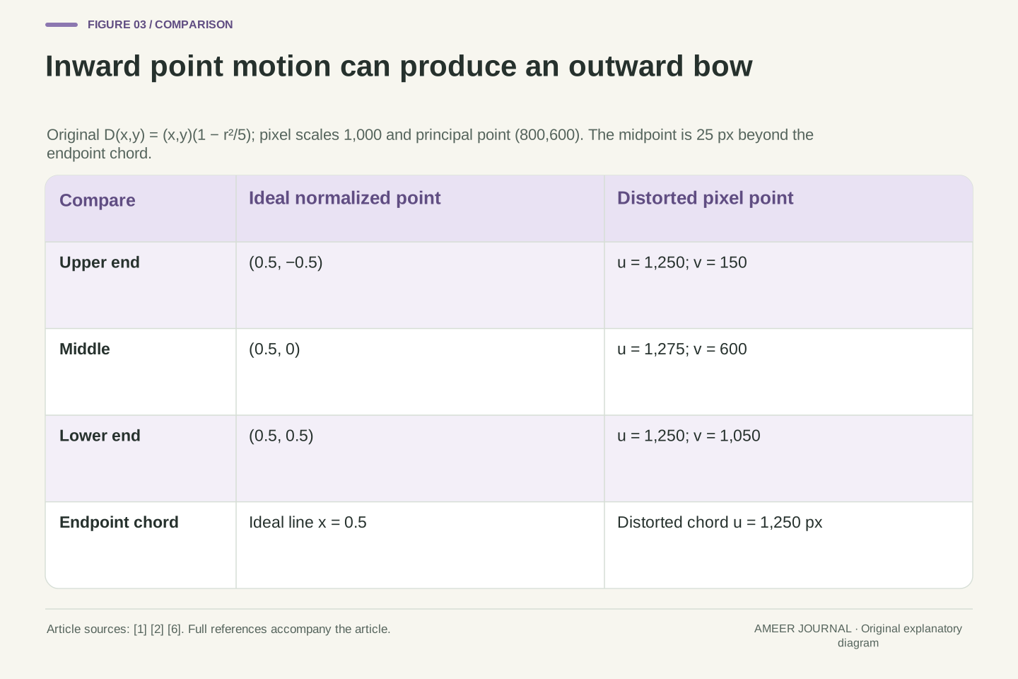
Take three ideal points on the vertical line x=0.5: their y coordinates are −0.5, 0 and 0.5. The two end points have squared radius 0.5, so their scale is 0.9. They move to (0.45, −0.45) and (0.45, 0.45). The middle point has squared radius 0.25 and moves to (0.475, 0). All three have moved toward the reference centre, but the middle point now lies farther right than the line joining the two ends.
Using our pixel scale, the end points are at (1,250, 150) and (1,250, 1,050), while the middle is at (1,275, 600). It sits 25 pixels outward from the vertical chord through the ends. There is no contradiction: inward displacement compares each point with its original location; outward bow compares the shape with the chord. Adobe describes barrel distortion through this bowed-line appearance. [6] Our calculation explains how that appearance can arise even while each selected point moves inward under the declared radial map.
Parameterize an ideal offset line by x=1/2 and select y∈{−1/2,0,1/2}. At the endpoints r²=1/2, giving D=(9/20,±9/20). At the midpoint r²=1/4, giving D=(19/40,0). These three transformed points are not collinear: the endpoint chord has x_d=9/20, while the midpoint exceeds it by 1/40. This is an original direct consequence of the declared map, not a fitted distortion measurement. The endpoints are symmetric about y_d=0, so their chord crosses that row at x_d=9/20. Comparing the midpoint with this chord therefore does not mix different vertical positions.
Converting through the fixed intrinsic scale gives endpoints (1250,150) and (1250,1050), and midpoint (1275,600). The chord-relative displacement is therefore 25 pixels. Each point's radial displacement is inward, but the line's midpoint bulges outward relative to its endpoints, consistent with Adobe's description of barrel-like line appearance. [6] The two statements use different references. Distinguishing point displacement from shape curvature avoids the mistaken inference that every point must move outward for a line to bow outward.
A straight line through the centre can stay straight
Now place the ideal line through the reference centre instead. For the horizontal line y=0, multiplying both coordinates by our positive radial scale leaves y at zero. Its points change their spacing, but they remain on the same horizontal line. The same reasoning applies to another line through the centre: all its points keep their original direction from that centre. Our model can therefore distort the image while leaving these particular lines straight.
This gives a useful limit on a visual check. Seeing one straight edge that crosses the centre does not prove the radial coefficient is zero. In our fixture, that observation fits both the zero-coefficient model and the model with coefficient −0.2. An offset edge provides different evidence because its points sit at different directions and radii, as the previous example showed. The point is to ask what a chosen observation can distinguish, rather than use any tidy-looking line as proof that every part of the image geometry is correct.
For a line through the distortion centre, write (x,y)=t(a,b) with a fixed direction (a,b). Then D(t a,t b)=t s(r)(a,b). Positive s(r) changes radial spacing but leaves the direction on that same line. In particular, y=0 implies y_d=0 throughout our domain. The result follows from the radial map's form; it does not require k_1 to vanish.
Consequently, collinearity of a single centre-crossing feature does not identify the coefficient in this example. Both k_1=0 and k_1=−1/5 preserve that line, although their point spacing differs. The offset line in the preceding section supplies a curvature witness that the central line lacks. This is a bounded identifiability observation about the selected feature, not a calibration algorithm or a recommendation to estimate a real lens from one edge. The geometry explains why the location and type of evidence matter when judging a correction.
The declared radius range is part of the model
Our example is restricted to normalized radii from zero to one. Within that region, the scale stays between 0.8 and 1, and increasing an input radius always increases the resulting radius. The mapping keeps the ordering of points along a ray, so one observed radius in its output range corresponds to one original radius. That property is useful when we ask to undo the mapping.
Extending the same polynomial indefinitely would change the situation. At input radius 1 it gives output radius 0.8, but at input radius 2 it gives only 0.4. The larger input has folded back toward the centre. Radius 2 lies outside our declared domain, and the example supplies no evidence that a real lens follows that extrapolation. A formula needs an applicable region as well as coefficients. Keeping that region visible prevents an apparently simple correction rule from becoming an unsupported claim about every corner or every possible field of view.
On 0≤r≤1, the scale s(r)=1−r²/5 is at least 4/5, and the radial derivative dr_d/dr=1−3r²/5 is at least 2/5. The radius map is therefore strictly increasing, with output interval [0,4/5]. Together with preserved direction and the fixed origin, this makes the declared radial map one-to-one on the disk. At the origin the angle is undefined, but only zero input radius produces zero output radius; it introduces no second point with the same mapped position. The derivative is an analytical check of our fixture, not evidence that a calibration implementation enforces such a condition.
Outside the chosen domain, the derivative changes sign at r=√(5/3). In particular, r_d(1)=4/5 but r_d(2)=2/5, demonstrating why unrestricted extrapolation would fail to preserve radial order. We do not extend the inverse beyond the stipulated usable region. A profile's mathematical family, coordinate convention and domain must be considered together; the existence of a polynomial expression does not establish its physical validity over an arbitrary field. Our later image-lookup examples remain within the declared region.
Undoing the point map requires its inverse
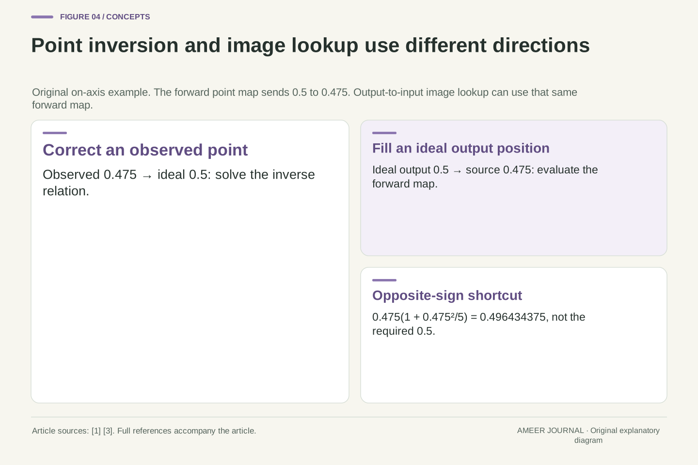
Suppose a measured point lies on the horizontal axis at normalized coordinate 0.475. Which ideal coordinate produced it? In our model, 0.5 is the answer because 0.5 multiplied by 0.95 equals 0.475. We are now going from the distorted observation back to the ideal point, reversing the relationship we used earlier. Simply changing the coefficient's sign is a tempting shortcut, but it asks a different mathematical question.
Try that shortcut explicitly: multiply 0.475 by one plus one-fifth of 0.475 squared. The result is 0.496434375, short of 0.5 by 0.003565625. At our scale, that difference is 3.565625 pixels. The shortcut used the observed radius inside the scale, whereas the original forward mapping used the ideal radius. Correct inversion must account for that dependency. This example does not rate any software's accuracy; it demonstrates why an opposite sign, without the inverse relationship, is insufficient even for a simple one-coefficient model.
For an observed on-axis coordinate x_d=19/40, solve x−x³/5=19/40 on the declared domain. The solution x=1/2 is verified directly, and the monotonicity established above gives uniqueness there. This is inversion of D. It is different from evaluating another forward polynomial whose coefficient happens to have the opposite sign. In the declared pixel coordinates, the observed point (1275,600) returns to ideal (1300,600). This names the input and output spaces before comparing their numerical difference.
The sign-flipped trial is (19/40)[1+(1/5)(19/40)²]=158859/320000=0.496434375. Its residual from the desired ideal coordinate is 1141/320000, or 1141/320=3.565625 pixels at f_x=1,000. The discrepancy arises because the radius used in the trial belongs to the distorted point. These exact fractions supply a counterexample to treating coefficient negation as an exact inverse. No iterative solver, tolerance or convergence result is asserted; the particular inverse solution is known because we constructed the original point.
An undistorted output can use the forward distortion formula
Producing an entire corrected image asks a different question from correcting one observed point. Start with a position in the desired output and ask where to obtain its value from the recorded image. OpenCV's geometric-transformation documentation describes this destination-to-source lookup. [3] For our correction, the output position represents an ideal coordinate, so the forward distortion rule tells us where that ideal point appeared in the distorted source.
For example, output pixel coordinate (1,300, 600) represents ideal point (0.5, 0). Our forward map sends it to (0.475, 0), corresponding to source coordinate (1,275, 600). The output can obtain its sample there. We have used the forward point-distortion formula as a backward lookup through the image. Both descriptions are correct because they name different directions: ideal-to-distorted coordinates and output-to-input sampling. Keep the output and source labels beside the arrows, and the apparent contradiction disappears.
Point correction maps an observed distorted coordinate through D inverse. Raster undistortion can instead iterate over ideal output positions and evaluate D to locate source samples. OpenCV documents geometrical resampling as destination-to-source lookup. [3] With unchanged intrinsic scale, no rectification rotation and our selected ideal output geometry, the sampling map is sourcePixel = K applied to D applied to normalizedOutput, where K denotes the stated zero-skew pixel conversion.
At output (1300,600), normalization gives (1/2,0); D gives (19/40,0); pixel conversion gives source (1275,600). Thus the physical distortion model's forward direction is the renderer's output-to-input direction. There is no need to negate k_1 for this lookup. Distinguishing these named interfaces is more precise than saying every correction must run an inverse formula. A different output matrix or rectification choice would change the complete sampling map, so this equality belongs to the explicitly unchanged output geometry.
A coordinate lookup still needs a sampling rule
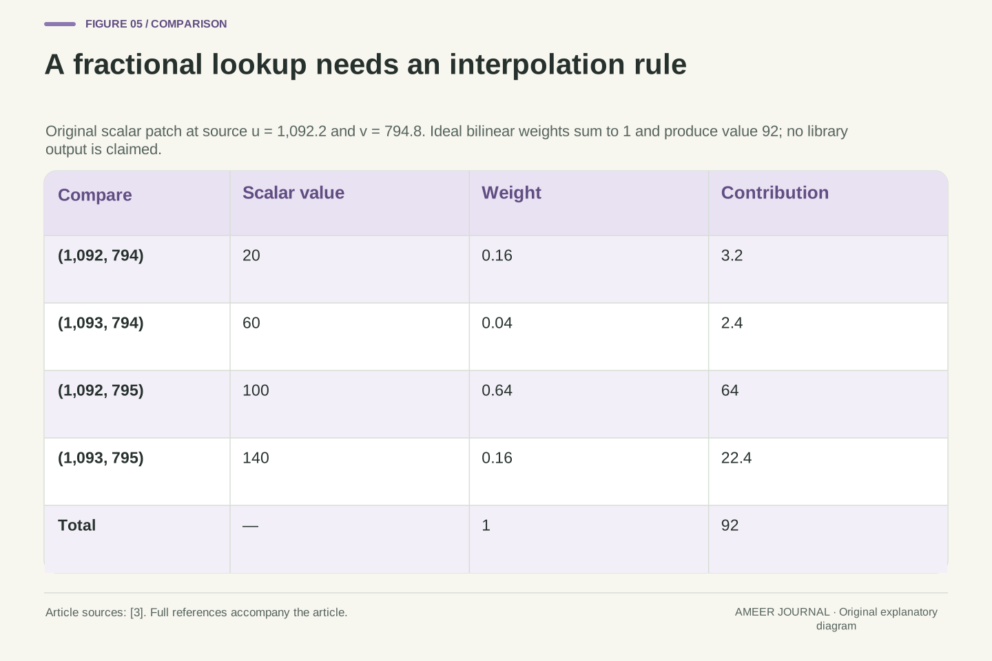
The source location need not land on an integer pixel position. Choose ideal output coordinates (0.3, 0.2). Their squared radius is 0.13, making our scale 0.974. The distorted coordinates become (0.2922, 0.1948), or source position (1,092.2, 794.8) in pixels. OpenCV separates this fractional-coordinate problem from finding the coordinate itself, and provides interpolation methods for estimating a value there. [3] A geometrically specified lookup has not yet selected that estimate.
For an original single-channel example, assign values 20 and 60 to the two neighbouring pixels on row 794, at columns 1,092 and 1,093. Assign 100 and 140 directly below them on row 795. Ideal bilinear interpolation uses the fractional offsets 0.2 across and 0.8 down, giving weights 0.16, 0.04, 0.64 and 0.16. The weighted value is 92. This is declared scalar arithmetic, not a measured colour result or a promise about an implementation's rounding. The interpolation estimates an output value from supplied samples; it does not make another observation of the scene.
For normalized output (3/10,1/5), r²=13/100 and s=487/500. Thus D=(1461/5000,487/2500)=(0.2922,0.1948), yielding source (1092.2,794.8). The corresponding ideal output pixel is (1100,800). OpenCV's remapping documentation distinguishes the coordinate map from the interpolation and border rules needed to obtain sample values. [3] This distinction remains relevant even when the continuous geometry is exact.
Take a hypothetical scalar patch with values a00=20, a10=60, a01=100 and a11=140 around that source location. Fractions α=1/5 and β=4/5 give bilinear weights (1−α)(1−β), α(1−β), (1−α)β and αβ, namely 4/25, 1/25, 16/25, 4/25. They sum to one and produce 92. This is ideal scalar interpolation without quantization, gamma interpretation or implementation-specific coefficient tables. It establishes the result of our chosen sampling rule, not a universal numerical output from OpenCV or recovery of finer scene information.
Output size and border policy are additional choices
A correction also needs a decision about the output's extent. MathWorks documents separate same, full and valid output-view options: matching the input dimensions, accommodating the input image, or retaining a valid cropped region. It also provides fill values when a mapped source location lies outside the input. [4] Those choices explain why two corrected outputs can have different boundaries even when they use the same underlying lens model.
Matching dimensions does not prove that each output position shows the same part of the source as before. Equally, a full view is not a promise that every output sample equals an original sample without interpolation. The useful comparison names the model, output geometry and sampling policy. Our numerical fixture kept the same scale and centre to isolate the radial effect; other choices must be stated separately. Adjusting a canvas or excluding an unsupported border changes presentation, but it does not physically move the camera or supply a new view behind an object.
The continuous map and destination sampling grid do not uniquely determine output extent or out-of-bounds handling. MathWorks undistortImage documents OutputView choices same, full and valid, together with FillValues and a returned output-intrinsics object. [4] These are implementation-defined controls in the retrieved documentation. Full coverage of the input image should not be interpreted as preservation of every discrete input value without resampling.
Our examples fix the ideal output scale and principal point, so their lookup equations remain simple. A different output geometry requires the corresponding intrinsic description, which MathWorks recommends using for subsequent geometric work. [4] The separate vehicle-camera guide develops crop-coordinate bookkeeping; no such coordinate-change example is needed here. The present distinction is that lens-model correction, output coverage and sampling are separate decisions. A changed border or canvas does not establish a changed physical viewpoint, and no wider output can validate extrapolation beyond a model's declared useful region.
A profile has to describe the image and the intended correction
A real editing application needs evidence for its chosen model. Adobe describes lens profiles identified using camera and lens metadata, with manual selection when a suitable match is not found automatically. It also notes that available profiles depend on whether the file is RAW or non-RAW. [6] Those are reasons to keep the camera, lens and input representation attached to the correction, instead of judging a profile only by whether its name looks familiar.
The same documentation discusses lens behaviour at different focal lengths, apertures and focus distances. [6] Our single coefficient cannot stand in for all of those conditions. For the invented example, we can verify the algebra exactly because we declared the model and inputs. For a photograph, the chosen model's applicability needs its own evidence. A useful comparison records which profile or parameters were applied, which geometry was requested, and which features were checked. That record separates a plausible visual improvement from a claim that every position or every later measurement has been validated.
Model applicability is distinct from algebraic correctness. Adobe's profile workflow uses camera/lens identification from Exif and permits explicit profile selection when automatic matching fails; available profiles can depend on RAW versus non-RAW input. [6] These are scoped workflow facts, not guarantees that a matching label establishes correct parameters for every processed image. The article's exact map is supplied as an assumption, whereas a practical profile must describe the actual representation being corrected.
Adobe also identifies focal length, aperture and focus distance as relevant conditions for lens behaviour. [6] Preserve such context when interpreting a profile or calibration record. Our finite-radius model demonstrates a geometric mechanism but supplies no measured fitting error or validity evidence for real equipment. Record the model family, coordinate normalization, parameter direction, applicable conditions and output choices together. That record makes it possible to distinguish an incorrect model selection from a different sampling or output-view choice without importing the vehicle article's separate pose-and-ground-plane assumptions.
Zero coefficients still need a model name
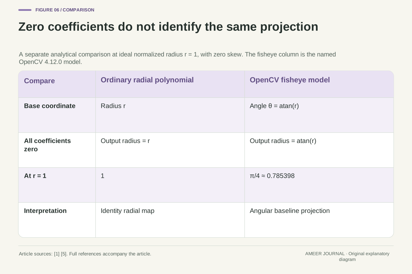
Finally, a coefficient has meaning inside a particular model. OpenCV's documented fisheye model begins with an angle obtained from the ideal radius, then applies its polynomial to that angle. [5] Our earlier ordinary radial polynomial begins with the radius itself. The two models can therefore use similar coefficient names while describing different baseline projections. Setting their coefficients to zero does not make their outputs automatically interchangeable.
At ideal normalized radius 1, the ordinary radial polynomial with zero coefficients returns radius 1. The named OpenCV fisheye model with all four coefficients zero returns an angle of π/4 radians, producing normalized output radius about 0.7854 when skew is zero. This separate comparison explains why zero is not a universal 'same geometry' setting. To interpret a lens correction, keep four things together: the coordinates, the model, the direction of the operation and the output sampling choices. Straightening a line is then a specific geometric result, with its viewpoint and remaining assumptions still visible.
OpenCV 4.12.0's fisheye model defines θ=atan(r), θ_d=θ(1+k_1θ²+k_2θ⁴+k_3θ⁶+k_4θ⁸), and the normalized distorted vector as (θ_d/r)(x,y) for nonzero r. [5] With all four coefficients zero and zero skew, its normalized output radius is θ=atan(r). By contrast, the ordinary radial polynomial with all coefficients zero has r_d=r. Similar parameter names therefore do not establish interchangeable parameterizations. The ratio atan(r)/r tends to one near the origin, so agreement close to the centre would not establish equality of the two maps across the image.
At r=1, the two zero-coefficient outputs are 1 and π/4≈0.785398 respectively. This is a direct analytical comparison of named models, not a fisheye-lens test or a proposed universal conversion. The correct interpretation must identify the projection family before treating zero coefficients as an identity. Combined with the preceding examples, the practical record is clear: specify coordinate normalization, mapping direction, model domain and raster/output policy. Those details explain both a straightened feature and the limits of what that correction establishes about the original viewpoint or captured information.
Sources & further reading
Explore the references behind this guide. External pages may change after our review.
- OpenCV: Camera CalibrationOpenCV · Accessed 7 Nov 2026
- What Is Camera Calibration? - MATLAB & SimulinkMathWorks · Accessed 7 Nov 2026
- OpenCV: Geometric Image TransformationsOpenCV · Accessed 7 Nov 2026
- undistortImage - Correct image for lens distortion - MATLABMathWorks · Accessed 7 Nov 2026
- OpenCV: Fisheye camera modelOpenCV · Accessed 7 Nov 2026
- Correct lens distortions in Adobe Camera Raw | Camera RawAdobe · Accessed 7 Nov 2026
Article updated 7 Nov 2026.
Found something we should revisit?
Good explanations get better with thoughtful feedback.