What you’ll take away
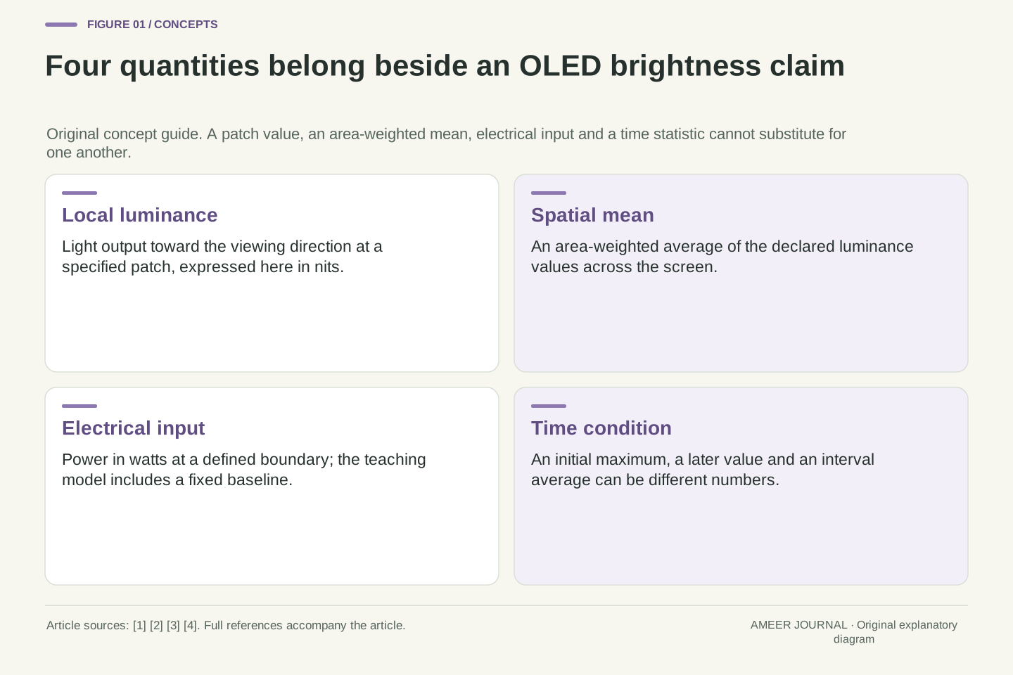
- A local peak, a spatial mean and a full-screen luminance value describe different quantities.
- In the hypothetical model, a local ceiling and a complete-screen power budget jointly limit the patch output.
- The surrounding field can change the available highlight budget even when the patch area is unchanged.
- An average loses brightness distribution, while a first peak does not establish a later or time-averaged output.
- Keep test version, pattern, duration, mode and evidence origin attached to each reported brightness value.
A bright highlight and a white page ask different questions
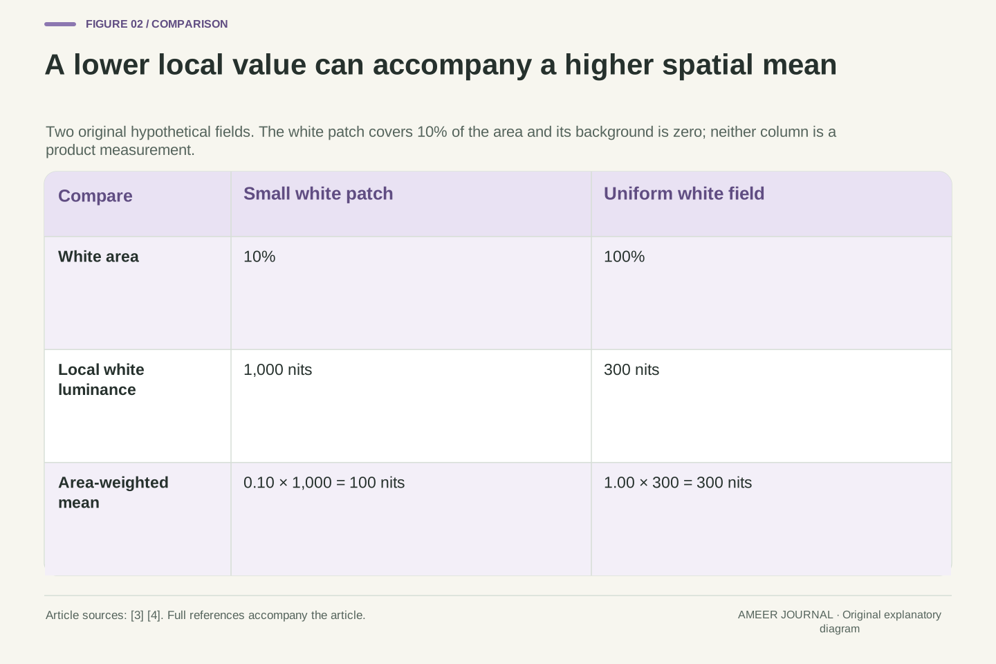
An OLED display can have a high number beside “peak brightness” without producing that same output across an entirely white screen. Imagine two hypothetical records: a white patch covering one tenth of the screen produces 1,000 nits, while a full white screen produces 300 nits. These records do not contradict each other. They describe different amounts of illuminated area. Microsoft's display documentation makes this distinction explicitly by providing separate maximum-luminance and maximum-full-frame-luminance fields. [3]
A nit is a unit of luminance, also written as a candela per square metre. [3][4] For this explanation, it describes the light leaving a displayed surface toward the viewing direction. It is not the screen's electrical power, and a high value at one small patch is not an average across the whole picture. We will follow invented numbers through those boundaries, then add background light and measurement time. None is a measurement of an actual monitor. The aim is to understand which conditions must accompany a brightness claim before two numbers can be compared.
A maximum-luminance value describes an output under particular spatial and operating conditions. It does not automatically specify the attainable luminance of a uniform full-frame field. Microsoft documents this distinction in DXGI_OUTPUT_DESC1: MaxLuminance is likely valid only for a small panel area, while MaxFullFrameLuminance addresses a colour filling the panel. [3] Our opening hypothetical records are a 10% white patch at 1,000 cd/m² and a full white field at 300 cd/m². Both can be internally consistent.
Luminance, expressed here in cd/m² or nits, remains distinct from electrical power and from an area-weighted mean of luminance samples. [3][4] All following calculations are original illustrative models for a fixed screen area, white spectrum and viewing direction. The declared power relation is a deliberately simplified scalar rule, not a measured efficiency curve or a manufacturer's control algorithm. Separately prescribed time records will add another measurement boundary. Keeping these definitions fixed allows us to establish what each number means without claiming that every OLED follows the same area curve or timing response.
Individual light emitters still share a complete-device budget
Apple describes OLED as emitting light through its pixels without a backlight. [1] That makes the picture's bright and dark regions relevant to the light-producing part of the display. However, separately controlled pixels do not imply an unlimited amount of power for every pixel at once. EIZO explains that increasing OLED image brightness increases power and heat, and that brightness limiting helps manage the resulting load. [2] The useful distinction is between where light is produced and what the complete display can supply.
Nor does a black image prove that the complete device consumes no electricity. Our coming model therefore includes an invented fixed ten-watt term for everything outside its variable light-production term. That number is a bookkeeping assumption, not a typical OLED specification. When the model's light-producing term falls to zero, its total remains ten watts. This small addition prevents two mistakes: treating all input power as light-producing power, and turning a statement about dark pixels into a battery-life claim about a whole laptop or television.
Self-emissive OLED operation removes the need for the separate backlight described in Apple's explanation. [1] It does not remove aggregate electrical or thermal constraints. EIZO identifies power consumption and heat generation as reasons for limiting brightness. [2] Those documented mechanisms motivate an accounting model; they do not supply the coefficients or control law we choose below. In particular, independent spatial addressability is not a statement that arbitrary simultaneous per-pixel outputs are feasible.
Define the modeled input boundary to include a constant P₀ and an image-dependent term. We assign P₀=10 W for illustration, without identifying it with a measured driver, processor or whole-product standby figure. A black light-production field leaves this baseline unchanged. Consequently, a percentage reduction in the variable term need not produce the same percentage reduction in total input. The distinction also avoids assuming that emitted luminance is itself electrical power. A conversion coefficient will connect the two only inside the stated fixed-condition model, where its units and scope can be inspected.
A ten-percent window refers to area, not both side lengths
A window percentage needs a geometric definition. Take an invented 1,920-by-1,080-pixel screen. It contains 2,073,600 pixel positions. A rectangle 384 pixels wide and 540 pixels high contains 207,360 positions, exactly ten percent of that total. Its width is twenty percent of the screen width and its height is fifty percent of the screen height. Multiplying those fractions gives the ten-percent area. The example is a geometric exercise, not a prescribed certification pattern.
Making both sides ten percent as long would instead create a 192-by-108 rectangle, only one percent of the screen area. This matters when interpreting a report that says “10% window.” For the original ten-percent area, assign the white patch 1,000 nits and everything else zero. Its area-weighted mean is 0.10 × 1,000 + 0.90 × 0 = 100 nits. A uniform 300-nit screen has a larger mean despite the lower local maximum. Neither mean alone predicts how bright the two pictures will feel to a viewer.
Let a denote the fraction of the panel area occupied by a specified uniform patch. For equal-area pixel positions, the 1,920×1,080 grid has N=2,073,600 positions. A 384×540 patch has 207,360, so a=1/10. The dimensional fractions are 384/1,920=1/5 and 540/1,080=1/2; their product is 1/10. A 192×108 patch has a=1/100 instead. No assumption about the shape of a VESA test window is being imported from this construction.
For uniform patch luminance Lw and uniform background Lb, define the spatial mean L̄=aLw+(1−a)Lb. Our 10% patch at 1,000 nits on the zero-luminance background gives L̄=100 nits. The uniform 300-nit field gives L̄=300 nits and a smaller local maximum. This arithmetic mean is an explicitly defined statistic, not a model of perceived brightness or a substitute for luminous flux. It also should not be equated automatically with a vendor's encoded average-picture-level percentage without its normalization and signal definition.
Give the power model its units before using its limit
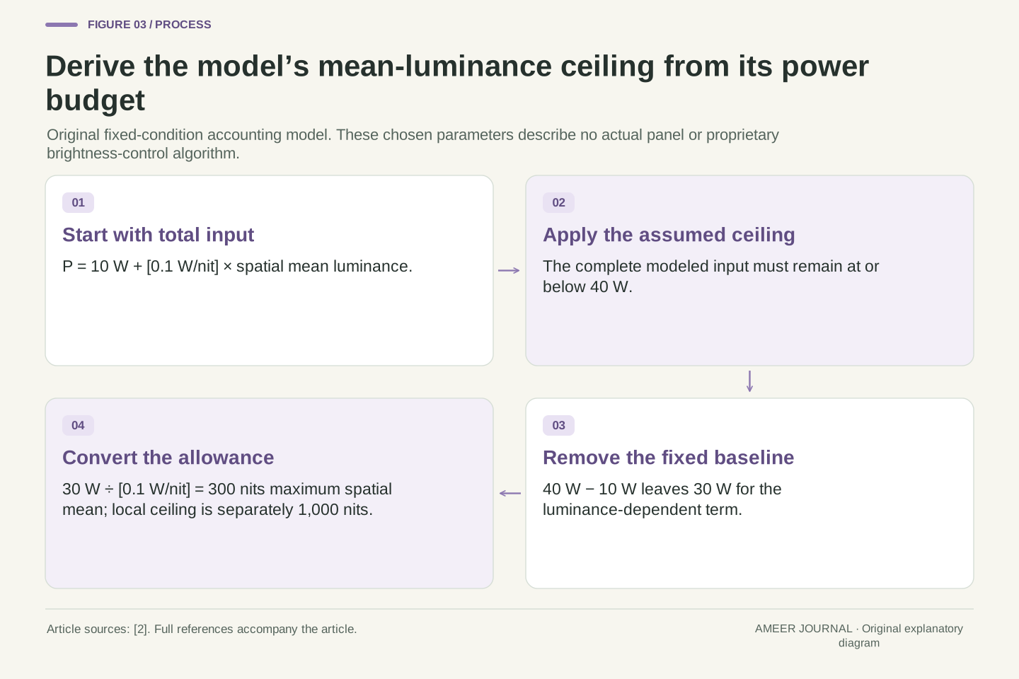
Now give our imaginary display a simple rule: start with ten watts, then add one tenth of a watt for each nit of the screen's area-weighted mean. At a mean of 100 nits, the total is 10 + 0.1 × 100 = 20 watts. At a mean of 300 nits, it is 40 watts. We choose 40 watts as the input limit and 1,000 nits as a separate local luminance limit. These are declared teaching assumptions, not values obtained from the source documents.
Subtracting the ten-watt baseline leaves thirty watts for the variable term. Dividing thirty by 0.1 gives a maximum permitted mean of 300 nits. That mean limit applies to the complete displayed field; the 1,000-nit limit applies locally. Both must hold at once. A small patch may satisfy both, while expanding the same requested output over the full screen would violate the first. The equation defines which outputs fit the budget. It does not decide how a real monitor chooses among the outputs that would fit.
Specify P=P₀+kL̄, with P₀=10 W, k=0.1 W/(cd/m²), input ceiling Pmax=40 W and local ceiling Lmax=1,000 cd/m². Because L̄ is in cd/m², kL̄ is in watts. The coefficient belongs to this fixed-area, fixed-spectrum teaching model; applying it to another panel size or colour composition would change the premises. EIZO's power/load discussion motivates examining a limit, but supplies none of these numeric assumptions. [2]
The aggregate inequality P≤Pmax becomes L̄≤(40−10)/0.1=300 cd/m². Independently, each region must remain at or below Lmax. Thus feasibility is the intersection of a spatial-mean constraint and a local constraint. At L̄=100, P=20 W; at L̄=300, P=40 W. We have specified no thermal state, temporal averaging, uniform-dimming rule or tone-mapping policy. The scalar bound can answer an accounting question about possible outputs without pretending to determine a complete display controller.
The active limit changes as the white area grows
Keep the background at zero and request the highest allowed white-patch output. At ten-percent area, the 1,000-nit local limit is reached while total model input is only twenty watts. At twenty-five-percent area, the same patch luminance gives a 250-nit mean and thirty-five watts. There is still room under the forty-watt ceiling. Enlarging the white area has used more power without yet requiring a lower patch value.
At half-screen area, 1,000 nits would give a 500-nit mean, which is too high. The maximum permitted patch value becomes 600 nits, bringing the mean back to 300. At full-screen area, the maximum becomes 300 nits. The changeover occurs at thirty-percent white area: 0.30 × 1,000 = 300. This piecewise result explains how both a high small-highlight number and a lower full-screen number can emerge from one set of assumptions. It is an upper boundary in our model, rather than a promise that a device always runs exactly on it.
With Lb=0 and a>0, the feasible patch maximum is Lw,max(a)=min(1,000,300/a). For a=0.10 and 0.25, the local ceiling is active: Lw,max remains 1,000 nits, while P is respectively 20 and 35 W. The local and aggregate constraints meet at a=300/1,000=0.30. The panel's total area is unchanged; a describes the fraction assigned to this white field.
For a=0.50, the aggregate ceiling sets Lw,max=600 nits, and for a=1 it sets 300 nits. Both have L̄=300 and P=40 W. Increasing area above the crossover changes the local upper bound inversely with a only because of the chosen linear power model and zero background. Below the crossover, that inverse relation is clipped by the local ceiling. At a=0, no white patch exists, so dividing by a is not meaningful. The derived boundary is conditional feasibility, not an empirically fitted OLED characteristic.
The unchanged highlight can lose headroom when its background lights up
Return to a white patch covering one quarter of the screen. On the black background, it could reach 1,000 nits in our model. Now keep its area fixed but set the other three quarters to 100 nits. The background contributes 0.75 × 100 = 75 nits to the complete-screen mean. Only 225 of the permitted 300 mean-nits remain available for the patch. Dividing that allowance by its one-quarter area gives a 900-nit patch limit.
The highlight did not grow, yet its permitted maximum fell by 100 nits. This is why a patch-size label alone does not fully describe a brightness test. Its surroundings also matter. Our calculation holds the background at 100 and asks what patch maximum remains feasible. A controller could instead choose to dim several regions or alter the requested mapping. EIZO documents different dimming treatments for its named professional monitor, illustrating why one allocation rule should not be silently assigned to every product. [2]
For a specified background, the aggregate condition gives Lw≤[300−(1−a)Lb]/a, provided the assumed background itself permits a feasible nonnegative patch output. Combine that bound with Lmax. With a=1/4 and Lb=100, the background contributes 75 cd/m² to L̄. The remaining patch contribution is at most 225, so Lw,max=min(1,000,225/(1/4))=900 cd/m². The resulting total is P=10+0.1(225+75)=40 W.
This is a constrained allocation holding Lb fixed, not a uniform multiplier applied to the entire image. It demonstrates why equal area does not guarantee an equal feasible patch value when the background changes. It does not establish which allocation an actual controller uses. EIZO's named CG3200X documentation distinguishes highlight and uniform dimming modes, which reinforces that policy boundary. [2] A brightness report therefore needs both the patch and its surrounding field, as well as the display's selected operating mode.
An average loses the distribution that produced it
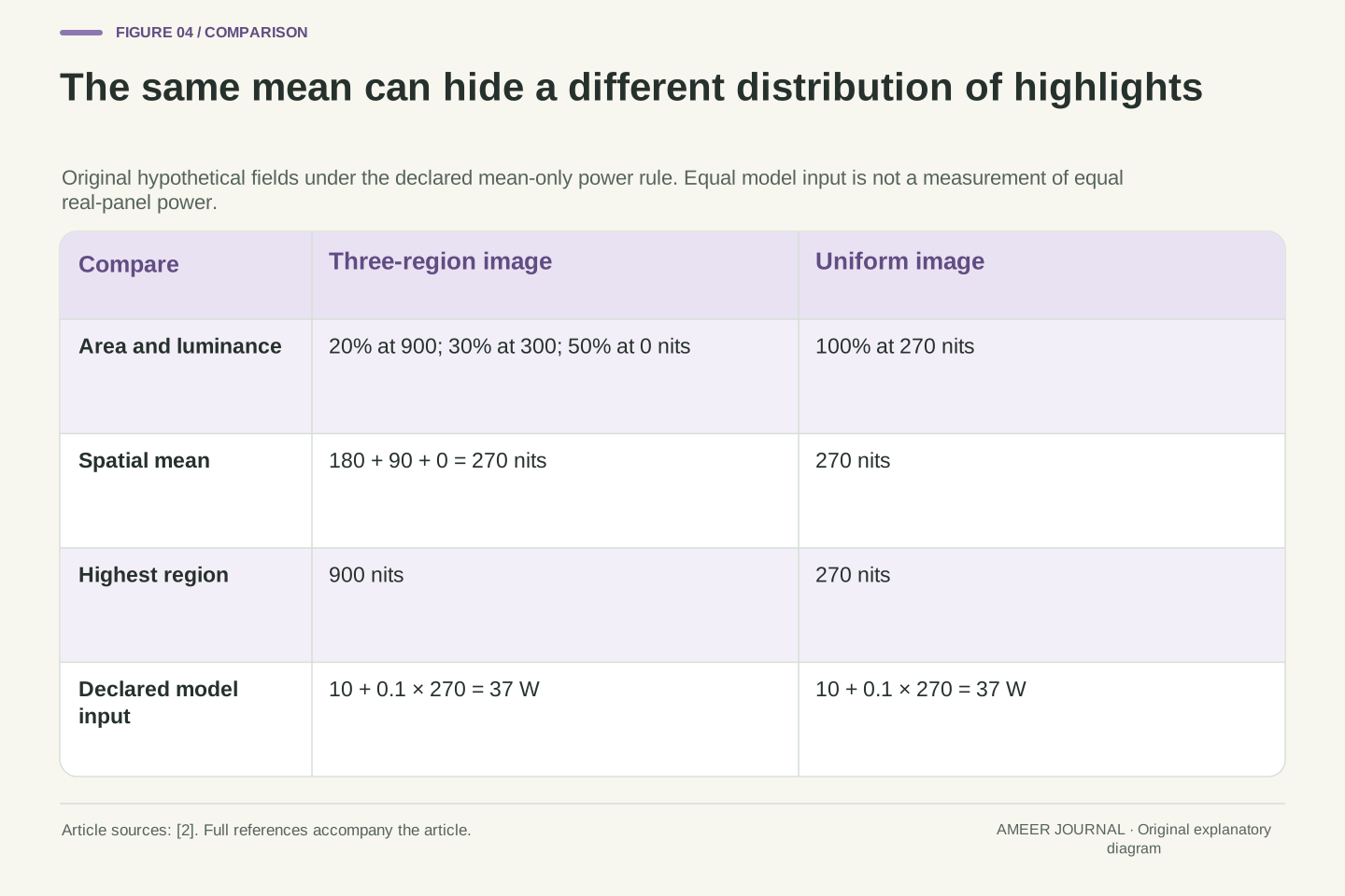
Consider another hypothetical picture: twenty percent of the screen is at 900 nits, thirty percent at 300 nits, and the remaining half at zero. Its mean is 180 + 90 + 0 = 270 nits. A completely uniform screen at 270 nits has exactly the same mean. Our power rule assigns both pictures thirty-seven watts. Yet the first has highlights more than three times as luminous as the uniform field, and the two images have very different bright-area distributions.
An average has kept one total while discarding the arrangement and local values. EIZO discusses this limitation of using a single average-picture-level summary and describes considering brightness distribution in its own control system. [2] The conclusion from our example is narrower: one scalar cannot reconstruct its contributing regions. It does not prove that these two patterns consume equal power on a real OLED, or that the same limiting action will occur. Those predictions would require evidence beyond the deliberately simplified mean-only model.
Let the regional area fractions be (0.2,0.3,0.5) and luminances be (900,300,0) cd/m². Their weighted mean is 270 cd/m². A uniform field at 270 has the same mean but a maximum of 270 rather than 900. Both satisfy the stipulated local and aggregate constraints, and P=10+0.1×270=37 W for either. Permuting the regional locations also leaves this scalar model unchanged.
The mapping from a luminance field to its mean is many-to-one. It removes local maxima, spatial arrangement and the distribution of area among levels. EIZO identifies this loss of distribution as a limitation of an average-based control input. [2] Our exact equality establishes indistinguishability under the model, not physical equality of every electrical or thermal quantity. A vendor's APL percentage additionally needs its own signal and normalization definition. We retain L̄ in measured-luminance units precisely to avoid passing an unstated encoded-picture statistic off as that defined spatial mean.
A first peak, a later value and a time average are different records
Area is not the only condition missing from a bare peak number. Imagine two separate invented time records for the same ten-percent patch. Record A shows 1,000 nits for the first two seconds and 300 nits for the following fifty-eight. Record B stays at 400 nits for the full minute. A has the higher initial peak, but B has the higher later value. Our earlier area-only equation does not predict these histories; here they are supplied as new assumptions.
The one-minute average of A is (2 × 1,000 + 58 × 300) ÷ 60, about 323.33 nits. B's average is 400. Calling A simply “1,000 nits” hides the time boundary, while calling 323.33 its sustained value would also be misleading: its later value is 300. VESA's criteria distinguish brief full-screen output from long-duration output. [4] A useful report states whether it recorded a maximum, a value after a specified hold, or an average over a defined interval.
Introduce prescribed temporal traces at one fixed 10% patch, with the rest of the field black. For A, Lw(t)=1,000 over 0≤t<2 s and 300 over 2≤t≤60 s. For B, Lw(t)=400 throughout. These are independent illustrative output records, not a thermal response derived from P=P₀+kL̄. In particular, neither a two-second protection timer nor a real panel time constant has been inferred.
The temporal patch mean for A is [2(1,000)+58(300)]/60=970/3≈323.33 cd/m². B's is 400. The ordering by maximum is therefore opposite to the ordering by this minute-long mean. A's terminal value is 300, which is yet another statistic. VESA separately names flash and long-duration full-screen tests. [4] That distinction motivates recording duration, but does not turn our time average into a VESA metric or our chosen two-second interval into its prescribed procedure. Spatial averaging and temporal averaging must retain their separate domains.
A named test gives the number a specific spatial and temporal context
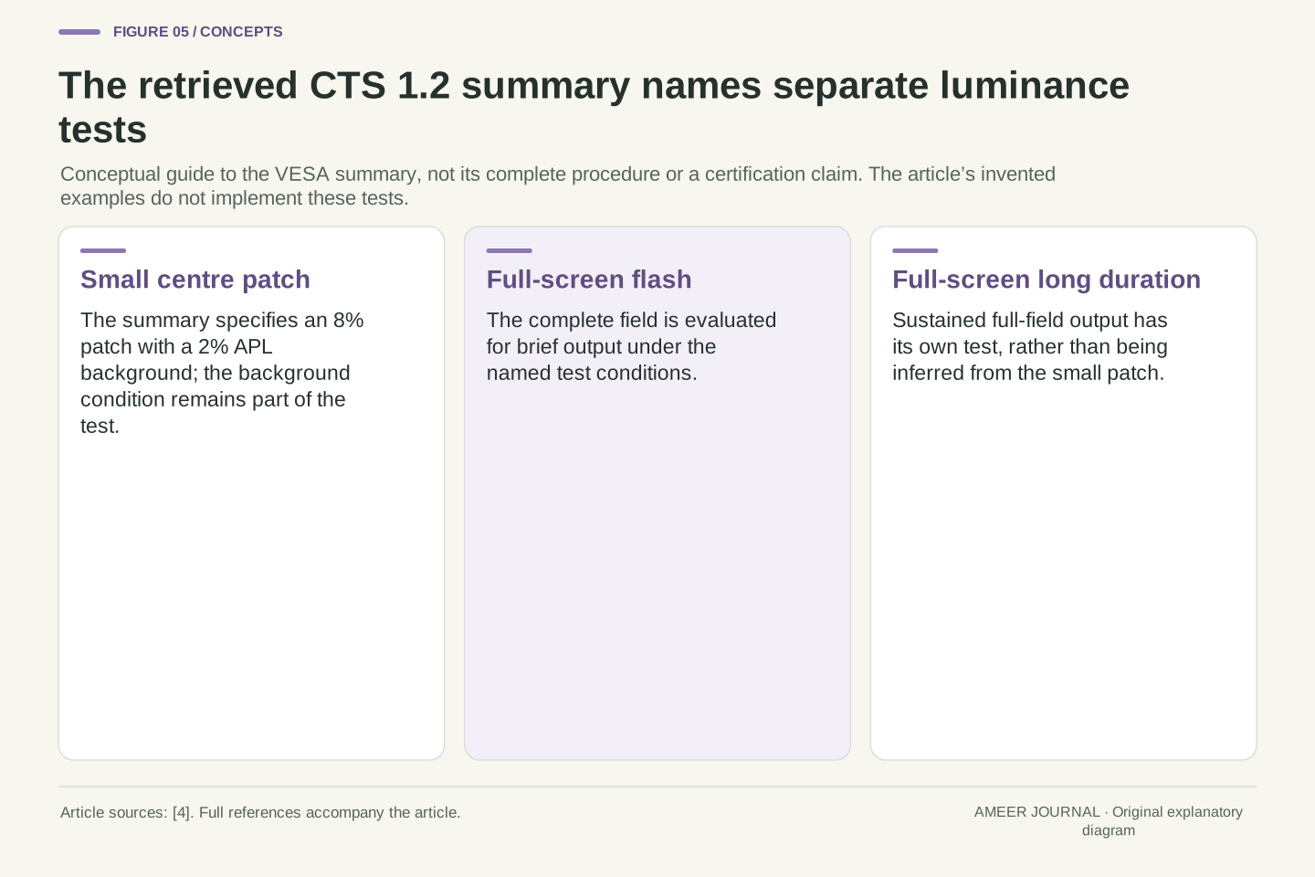
The retrieved VESA DisplayHDR CTS 1.2 summary specifies an eight-percent centre patch with a two-percent APL background, alongside separate full-screen flash and long-duration tests. [4] That small-patch description is different from our ten-percent patch on a zero background. It also does not mean that the background is simply two percent of the patch's measured nits; the summary's APL label belongs to its defined test conditions. Our examples are not certification tests.
A comparison should therefore retain the actual test name and version rather than replace them with “peak.” Ask whether both values used the same patch area, background, duration and operating mode. If those differ, the results may both be valid while answering different questions. The public summary also names black-level and colour evaluations. [4] A white-luminance result alone cannot establish success in those other evaluations. Reading the conditions is what turns a large number into useful evidence, without requiring a reader to treat every possible display property as one ranking.
The actual retrieved CTS 1.2 summary labels its small-area measurement as an 8% centre patch with a 2% APL background and separately lists full-screen flash and long-duration luminance evaluations. [4] Preserve the version and the full condition association. The background APL label is not converted here into an unprovided absolute luminance. Only the public summary was read; detailed conformance procedures from the complete CTS are not claimed.
Our original 10% geometry, linear power budget and minute-long traces implement none of those named tests. They explain why changing a measurement boundary matters. A like-for-like comparison must establish the relevant test conditions before attributing a numerical difference to the devices. Other summary categories include black-level and colour evaluations. [4] A scalar white-luminance measurement does not determine those results, even when a certification scheme groups several requirements under one designation. This also prevents treating a guessed full-screen value as a substitute for the actually reported small-patch measurement.
A software capability field is not a live light-meter result
Microsoft's MaxLuminance and MaxFullFrameLuminance fields carry different area meanings. The documentation says these values usually come from display identification data, or sometimes an override. [3] They help software understand a display description. Reading one field does not mean a light meter has just measured the current white patch, nor does it reveal what happens at every intermediate window size or after every possible duration.
Suppose a record contains the same 1,000 and 300 numbers used earlier. Those two values still do not establish our ten-watt baseline, our thirty-percent crossover, or our response to a 100-nit background. Many different curves could share the same two endpoints. They also do not identify why a particular application currently appears dimmer. Keep the capability description beside, rather than in place of, an observation that specifies what was displayed and when it was measured. That separation makes a discrepancy a question that can be investigated, instead of an automatic conclusion that a specification is false.
DXGI_OUTPUT_DESC1 exposes MaxLuminance and MaxFullFrameLuminance with their documented spatial distinction. Microsoft states that these values generally originate in EDID or an override. [3] They are capability-description fields, not samples from an instrument observing the current frame. The API documentation does not provide a universal function Lmax(a,t,background,mode) for every connected display.
Even if the described endpoints were 1,000 and 300 cd/m², they would underdetermine the interior of such a function. Our piecewise boundary required the additional local ceiling, linear coefficient, baseline, power ceiling and background assumptions. Another model could match two endpoints while differing elsewhere. A report should therefore identify whether its number is advertised, described by an interface or actually observed under a stated pattern. None of those categories should be silently substituted for another. This is an evidence distinction, not a claim that every EDID value is inaccurate or that every visible difference represents hardware failure.
A visible brightness change does not identify its cause by itself
Dell documents pattern-dependent luminance changes specifically for OLED versions of the Precision 5540 and XPS 15 7590. Its explanation relates the change to the proportion of white pixels in the image. [5] That is a concrete example of a loading effect, not proof that every OLED uses the same calculation or behaves identically in every application. Even its windowed-content context belongs to those named products.
Other adjustments answer different inputs. Apple describes ambient-light auto-brightness and separate per-pixel adjustments based on usage for its named iPhone displays. [1] A dimmer image alone does not tell you which input or control changed. A useful observation records the same content, surrounding light, display mode and elapsed time before attributing the change to area loading. This is a way to interpret a record, not a request to disable protection or leave a bright static pattern running. Keep the manufacturer's supported operating guidance with the actual product.
Dell's article scopes a pattern-dependent loading effect to OLED configurations of the Precision 5540 and XPS 15 7590, describing on-pixel ratio in terms of white-pixel proportion. [5] That implementation account supports the existence of the documented behaviour; it does not validate our coefficients, define all manufacturers' APL metrics or establish a universal output curve. The named models and source scope remain attached to the claim.
Ambient adaptation, usage-based pixel adjustment and content-dependent loading are different possible control inputs. Apple's support document describes the first two for its named displays. [1] Observing a luminance reduction without holding relevant conditions fixed cannot uniquely identify the responsible mechanism. Record content geometry, mode, environment and timing when interpreting an existing observation. This article does not prescribe service-menu changes, protection overrides or endurance experiments. Its purpose is to prevent a single visible symptom from being treated as a complete diagnosis when several documented mechanisms can affect output.
Read a brightness claim as a complete measurement sentence
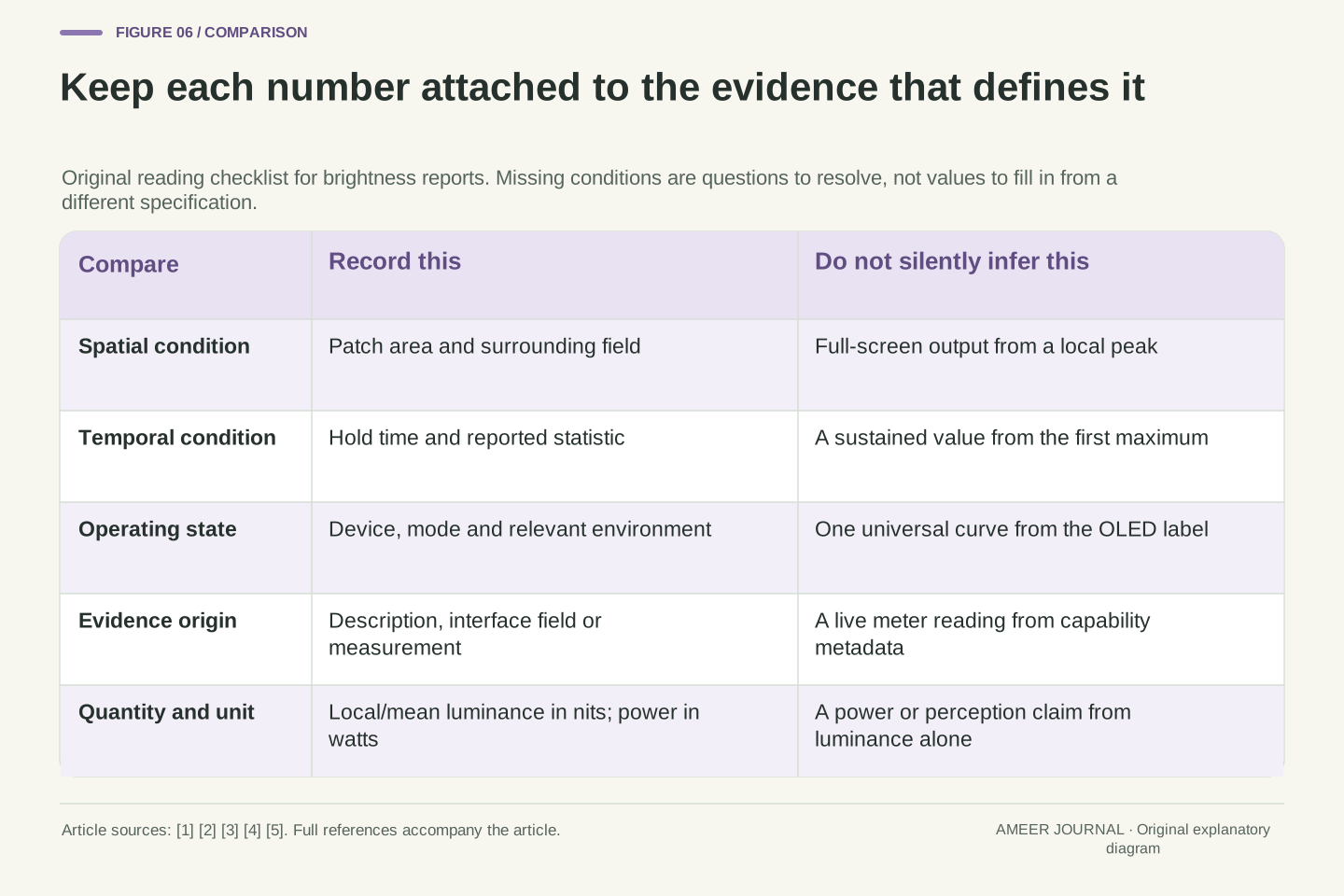
A useful statement names the device and mode, the patch area, the background, the time condition, the measured quantity and where the value came from. For example, our invented first record says that a ten-percent white patch on a zero background has a local value of 1,000 nits under its stated conditions. It does not say that the whole screen averages 1,000 nits, uses 1,000 watts, or holds that output for any chosen duration. Adding those missing claims would change the record.
When two reports disagree, first ask whether they describe the same experiment. Then check whether one reports a local peak while the other reports a full-screen value, or whether one captures a brief maximum while the other waits. If the conditions match and the results still differ, the difference deserves further evidence. If they do not match, preserve both records with their limits. That approach makes the small-highlight number and the white-page number intelligible parts of a display description, rather than forcing them into a single brightness promise.
Represent the comparison record as a tuple containing device/configuration, spatial pattern, background, temporal condition, statistic and evidence origin. The tuple need not be a new software format; it is a discipline for preserving the variables that qualify a numerical result. Our examples demonstrate why removing any of several entries permits incompatible interpretations. The same local peak can coexist with different spatial means, and the same peak can coexist with different time means.
A justified comparison aligns the relevant tuple entries before interpreting a residual difference. Capability metadata may help describe the system, but it does not supply missing instrument conditions. Likewise, a mean-only power example cannot establish a proprietary dimming policy or a complete luminance envelope. Use the actual reported quantity for the conclusion it supports. That leaves room for both a strong localized highlight and a lower sustained full-field output, while keeping performance, colour accuracy, power consumption and operating history as distinct questions that require their own evidence.
Sources & further reading
Explore the references behind this guide. External pages may change after our review.
- About the Super Retina display and Super Retina XDR display on your iPhone – Apple Support (AU)Apple Support · Accessed 7 Nov 2026
- EIZO Monitor Knowledge: OLED and ABLEIZO · Accessed 7 Nov 2026
- DXGI_OUTPUT_DESC1 (dxgi1_6.h) - Win32 apps | Microsoft LearnMicrosoft Learn · Accessed 7 Nov 2026
- Performance Criteria 1.2 TB1400 260708 - VESA Certified DisplayHDR™VESA DisplayHDR · Accessed 7 Nov 2026
- Brightness Changes on Precision 5540 or XPS 15 7590 | Dell CanadaDell Technologies Support · Accessed 7 Nov 2026
Article updated 7 Nov 2026.
Found something we should revisit?
Good explanations get better with thoughtful feedback.