A battery can have been warmed earlier and still be cooler than intended when the car reaches its next stop. That makes preconditioning a timing question as well as a heating question. The cited U.S. Model S manual connects preparation with departure scheduling and navigation to charging stops. The cited 2026 Hyundai U.S. manual page also describes conditioning with an expected charging-station arrival in mind. These are examples of particular documented controls, not promises about every vehicle. [1][2]

Conditioning does not always mean warming. Hyundai's page describes operation when the battery is too cold or too hot, subject to equipment and operating conditions. [2] Our question here is narrower: when warming is needed, why can starting earlier, stopping earlier and arriving earlier produce different results? A target temperature, the present thermal state and the time available each supply different information.

We will compare three schedules using one deliberately simplified mathematical battery body. It is an explanatory model, not a test of either manufacturer's car. Every temperature, heat capacity, power and duration in the calculations is assigned for this lesson. In particular, its 18°C target is not a recommended operating temperature. The useful result is the reasoning about timing, heat loss and energy boundaries.

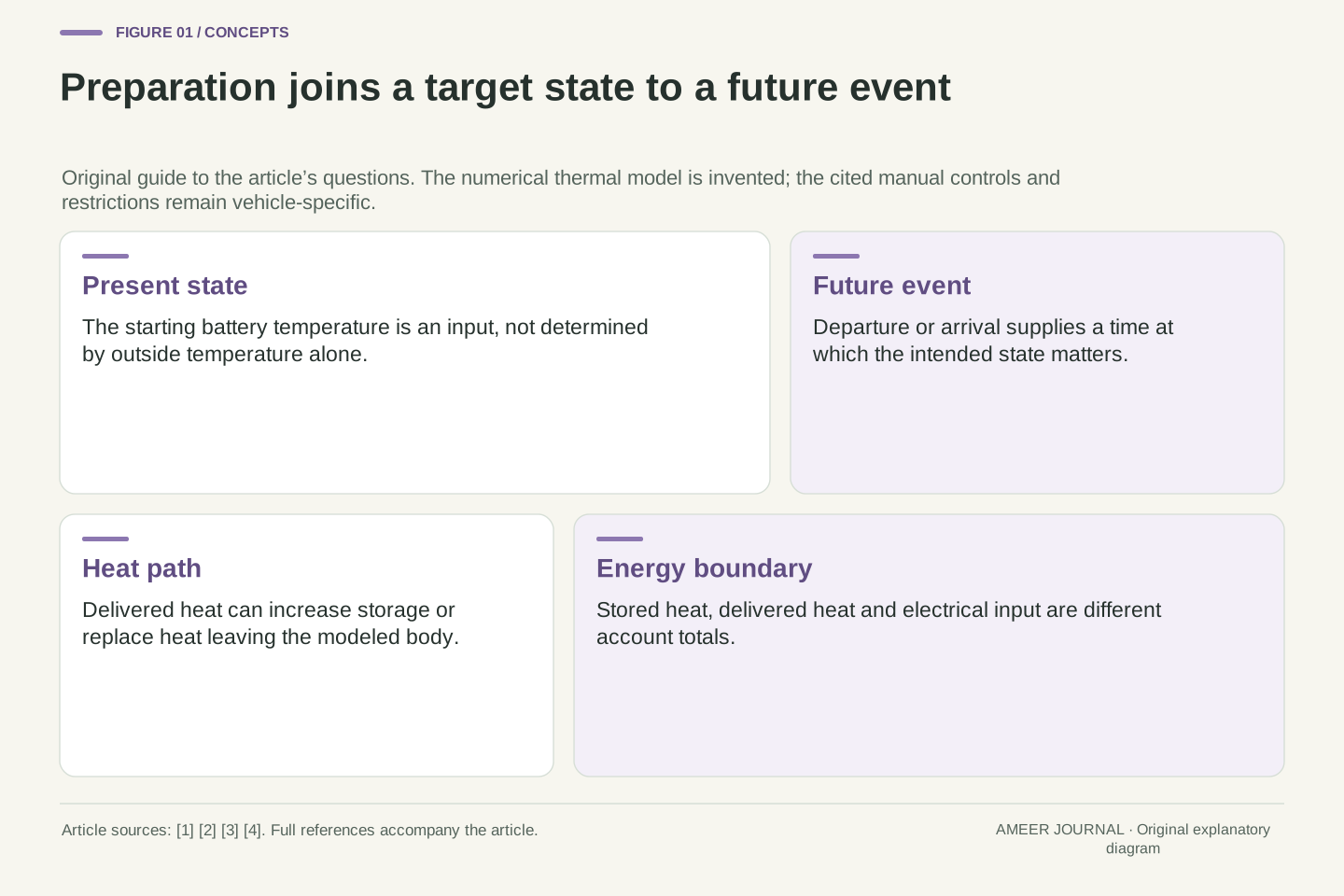
Preconditioning is a state-preparation problem with a future event: departure or arrival at a charging location. The Model S manual describes scheduled preparation and navigation-linked battery warming; the cited 2026 Hyundai U.S. topic describes arrival-aware conditioning and states equipment, charge-state and thermal restrictions. Those retrieved manual contexts establish why timing belongs in the question without defining a universal controller or feature set. [1][2]

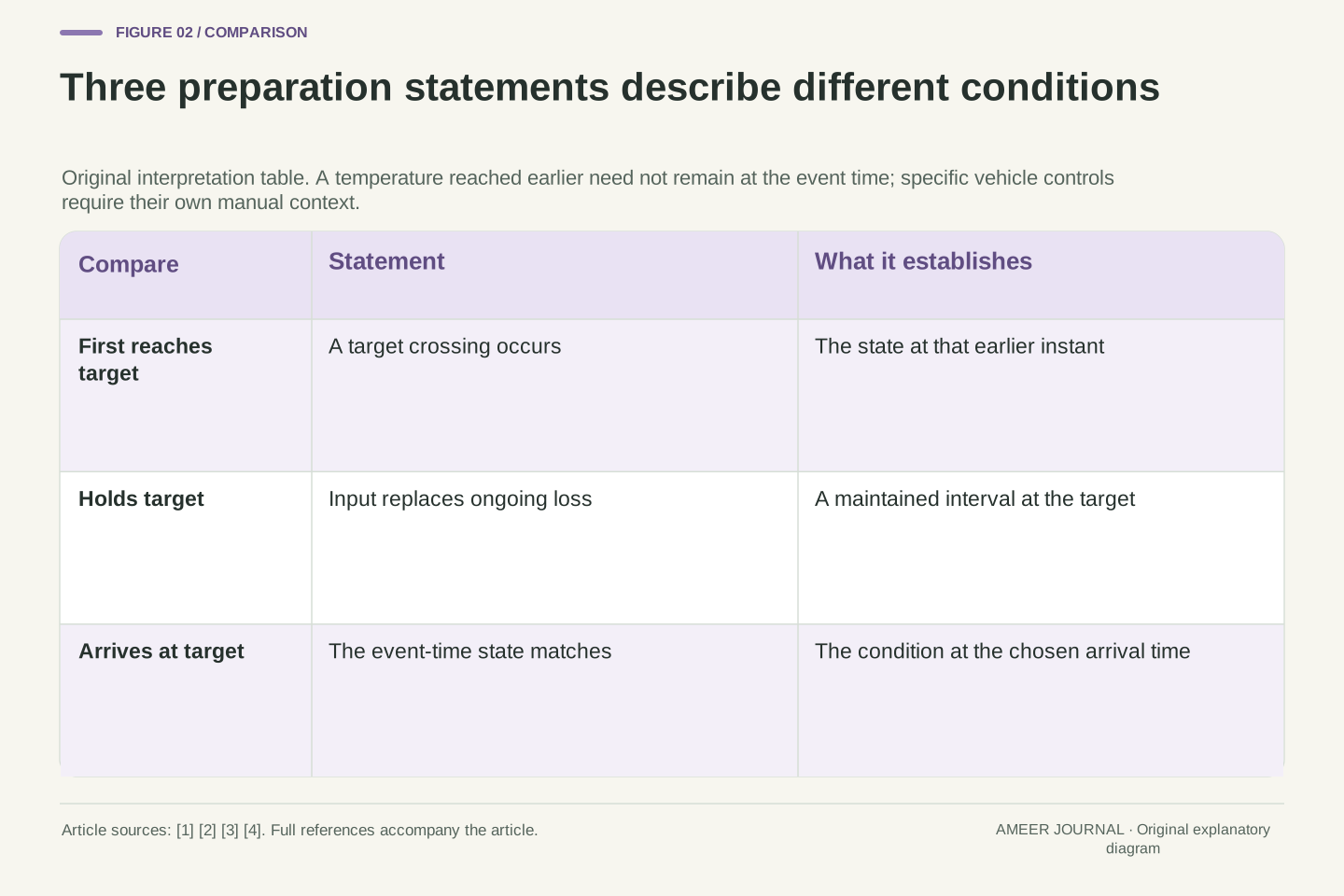
The Hyundai description includes both excessively low and high battery temperatures. [2] This article isolates a warming case and distinguishes three quantities: first passage through a target, maintenance of that target, and state at the event time. Achieving the first does not establish the third if heat subsequently leaves the body. A displayed start time alone therefore leaves the intended thermal outcome underspecified.

All following numerical parameters belong to an original, single-state teaching model. They are neither fitted vehicle data nor a simulated manufacturer controller. We choose a 45-minute event horizon and an arbitrary 18°C target under a 0°C ambient. No charging-power prediction follows from meeting that target; the calculation supplies only the defined thermal state and the energy transfers required by its equations.

Picture a single body that can store thermal energy. A heater delivers energy into it, while a heat path lets energy leave for the colder surroundings. MathWorks' thermal-mass documentation relates the net incoming heat rate to temperature change. Its thermal-resistance documentation relates heat flow to a temperature difference. Combining those two ideas gives a small model whose energy account we can follow. [3][4]

Assign the body a heat capacity of 0.1 kilowatt-hours per degree of temperature rise. Keep the surroundings at 0°C. Let each degree above the surroundings produce a heat leak of 0.1 kilowatts, and let the heater deliver up to 6 kilowatts of heat. The starting body temperature is also 0°C. These numbers define the example; the unit kilowatt-hour describes energy here, not a battery's electrical charge.

The single body has just one temperature. We have deliberately left out different cell temperatures, coolant temperatures, cabin demand and heat generated by driving. This makes the timing comparison readable, but it does not let a real coolant reading stand in for every cell. Within our chosen boundary, heater input minus outward heat flow is exactly the rate at which stored thermal energy changes.

Let θ=T−Tₐ be temperature rise above a fixed ambient Tₐ=0°C. Set thermal capacity C=0.1 kWh/K, heat-leak conductance G=0.1 kW/K and delivered heater power 0≤P≤6 kW. For the main cases θ(0)=0. With time measured in hours, the model balance is C dθ/dt=P−Gθ. Each term on the right is a heat-transfer rate in kW. [3][4]

The storage term is the constant-mass thermal relation with C=mc. The leak follows a constant equivalent resistance R=1/G: heat flow equals temperature difference divided by resistance. MathWorks uses Q for a heat-flow rate in these equations; here P and Gθ identify the two rates separately. Neither C nor θ is electrical state of charge, and kWh/K is a thermal-capacity unit. [3][4]

Assume one uniform model state, fixed parameters and no other heat source or storage node. Constant G is an assigned equivalent path over this calculation, not a claim that every real heat-transfer mechanism is linear at all temperatures. This boundary intentionally excludes spatial gradients and driving heat so that timing changes can be attributed to the declared input schedule.

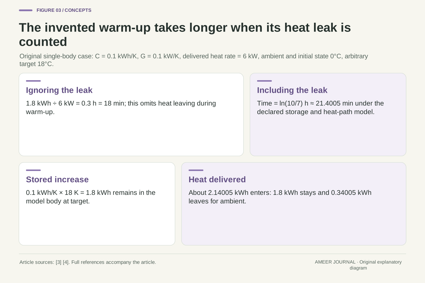
Raising this body from 0°C to 18°C adds 0.1 times 18, or 1.8 kilowatt-hours, to its thermal store. That is the change remaining in the body when it reaches the target. It is not necessarily all the heat that had to enter, because some could have left during the warm-up. The storage and heat-path relations describe these as separate parts of the account. [3][4]

At 18°C, the body is 18 degrees warmer than the surroundings. Its assigned leak is therefore 0.1 times 18, or 1.8 kilowatts. The matching numerals can be misleading: 1.8 kWh is an energy amount, whereas 1.8 kW is an ongoing rate. Holding the temperature for another half-hour would require 0.9 kWh of replacement heat under these unchanged conditions.

A steady temperature can thus hide continuous energy transfer. Supplying 1.8 kW at the target replaces the 1.8 kW leaving it, so the thermal store stops growing. Supplying nothing instead lets the body cool. The question 'Has it reached 18°C?' leaves open which of those two things happens next.

For fixed C, the stored-energy increase is ΔU=CΔθ. Heating from θ=0 to θ*=18 K therefore gives ΔU=1.8 kWh. At that state, the outward rate is Gθ*=1.8 kW. These quantities happen to share a numerical value because of our parameters, but they differ dimensionally and answer different questions. The storage and resistance equations require both. [3][4]

Holding θ constant makes dθ/dt=0, so P_hold=Gθ*. Over an additional interval Δt, replacement heat is H_hold=Gθ*Δt. For Δt=0.5 h, H_hold=0.9 kWh while ΔU during that hold is zero. All of the added heat crosses the outward boundary; none increases the model's thermal store.

The distinction also fixes the meaning of 'enough heat.' A 1.8-kWh increase in stored energy is necessary to reach the target from the stated initial condition, but an input account must additionally cover losses during the path. Conversely, a 1.8-kW source can balance the target's eventual loss without necessarily bringing a colder body to that exact target in finite time.

At the start, the body and surroundings have equal temperatures, so the model's outward leak is zero. All 6 kW initially increases its thermal store. As the body warms, the leak grows. Near the 18°C target, 1.8 kW leaves while 6 kW arrives, leaving only 4.2 kW to continue raising the temperature. The warming rate changes even though the heater output is constant. [3][4]

If we ignored the leak, dividing the required 1.8 kWh by 6 kW would give 0.3 hours, or 18 minutes. Solving the changing heat account instead gives about 21.4005 minutes to reach the target. The additional time comes from replacing heat that escapes during warming. It is not a mysterious delay added by a controller.

This calculation explains why a heating-power label and a desired temperature rise cannot determine preparation time by themselves. The initial temperature, thermal storage and heat path also matter. The Model S manual similarly says preparation time depends on outside temperature and other factors; its vehicle-specific guidance should not be replaced with our invented 21-minute result. [1]

For constant P, the differential equation has solution θ(t)=P/G+(θ₀−P/G) exp(−t/τ), where τ=C/G=1 h. With P=6 kW and θ₀=0, θ(t)=60 K[1−exp(−t/(1 h))]. The exponential's argument is dimensionless, and 60 K is this input's equilibrium rise in the fixed model, not an assigned operating target. [3][4]

Set θ=18 K. Then exp(−t/τ)=0.7 and t_w=ln(10/7) h=0.3566749439 h, approximately 21.4005 minutes. Neglecting the leak gives Cθ*/P=0.3 h, which is too short. The instantaneous net heating rate falls from 6 kW at the start to 4.2 kW at first target crossing.

A specified heater rate consequently does not fix a unique warm-up duration without a state and path model. Changes to initial temperature, capacity or conductance alter the result. Manufacturer guidance also recognizes condition-dependent preparation time. [1] Our analytic time belongs only to the declared parameters; it is not a timing calibration for either cited vehicle or an instruction to override its controls.

The heater runs at 6 kW for about 0.356675 hours. Multiplying those values gives approximately 2.14005 kWh of heat delivered during warm-up. Of that amount, 1.8 kWh remains as the body's increased thermal store. The remaining 0.34005 kWh has gone to the surroundings. The account closes: incoming heat equals stored increase plus outgoing heat. [3][4]

It would be wrong to label the full 2.14005 kWh as stored heat. It would also be wrong to call the 0.34005 kWh a separately measured electrical conversion loss. We have so far described only heat delivered into the body and heat leaving that body. The electricity used to produce or deliver the heat has not yet been specified.

This first warm-up becomes a reusable building block. Moving the same warm-up later will preserve its input and loss if it still starts at 0°C under the same surroundings. Adding a holding period changes the heat needed after that building block. Turning the heater off changes the final stored amount. Those are different extensions of the same initial calculation.

Integrating the input gives H_w=P t_w=2.1400496636 kWh. The stored increase is Cθ*=1.8 kWh, leaving L_w=H_w−Cθ*=0.3400496636 kWh. Directly integrating Gθ(t) over the warm-up yields the same outward transfer, independently closing the differential and interval accounts. [3][4]

The energy balance is H_w=ΔU+L_w. There is no electrical-conversion term in this particular boundary: P is already delivered thermal power. Introducing such a term later requires a wider input account and an explicit destination for the difference. It cannot be silently identified with L_w, because L_w is the modeled body's leak to ambient after heat has crossed its input boundary.

Time translation alone leaves this warm-up unchanged when the initial state and boundary conditions remain identical. A delayed start at ambient therefore retains H_w and L_w. Holding after warm-up adds a new interval with zero storage change, whereas coasting adds an interval with negative storage change. Comparing schedules requires accumulating these interval accounts to the same arrival time.

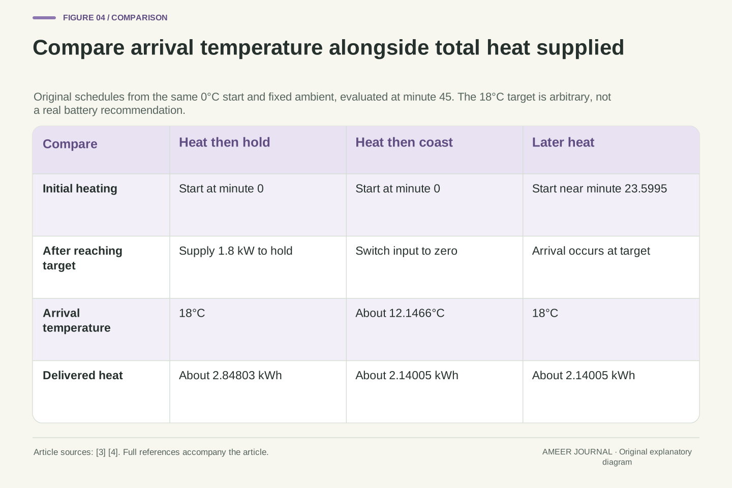
Our first schedule starts heating immediately. It reaches 18°C after about 21.4005 minutes, then keeps that temperature until the planned arrival at minute 45. The remaining holding period lasts about 23.5995 minutes. During the hold, the heat input drops from 6 kW to 1.8 kW so that it exactly replaces the ongoing leak.

That holding period needs approximately 0.707985 kWh of additional heat. Adding the warm-up's 2.14005 kWh gives 2.84803 kWh delivered in total. At arrival, the body still has only the original 1.8-kWh stored increase. The total outward transfer is now about 1.04803 kWh, because the body has spent extra time warmer than its surroundings.

The early start has bought time at the target, not a larger final thermal store. That can matter if the intended event moves earlier. It also has a cost under this model: replacing heat throughout the waiting period. Calling the whole interval a 6-kW heating session would miscalculate both input and temperature, because the schedule explicitly changes power after reaching the target.

For schedule A, apply P=6 kW from t=0 to t_w, then P=Gθ*=1.8 kW until t_a=0.75 h. The holding duration is t_a−t_w=0.3933250561 h. Exact modulation at the target makes θ(t)=18 K throughout this second interval; continued 6-kW input would define a different trajectory.

The added heat is H_hold=1.8 kW×0.3933250561 h=0.7079851009 kWh. Total delivered heat is H_A=2.8480347645 kWh. Since arrival storage is Cθ*=1.8 kWh above the initial reference, cumulative outward transfer is L_A=1.0480347645 kWh. The warm-up and hold intervals satisfy the same balance separately and together. [3][4]

This schedule establishes a period of target attainment before the event rather than a surplus final temperature. It spends heat maintaining that margin against earlier arrival. There is no assumed tariff, electrical supply source or charge-rate reward in H_A. The relevant comparison is between equal final thermal states with different input histories, while retaining the value of any earlier readiness as a separate scheduling consideration.

For the second schedule, keep the same immediate warm-up but switch the heater off at 18°C. The body then spends the next 23.5995 minutes cooling. Its heat leak becomes smaller as its temperature approaches the surroundings, so it does not lose the same amount every minute. The thermal-storage and heat-path equations together describe this slowing change. [3][4]

At minute 45, the calculated temperature is approximately 12.1466°C. The schedule used the same 2.14005 kWh as the original warm-up, but only about 1.21466 kWh remains as increased thermal storage at arrival. Cumulative heat lost is about 0.925393 kWh. The body did reach 18°C earlier; that statement is true, but it does not describe the event-time state.

This is why saving the holding heat cannot be counted as an equal-outcome improvement. The early-hold and early-coast schedules deliver different arrival temperatures. A useful comparison keeps both columns visible: total heat supplied and temperature at the intended event. Choosing only the lower heat number would hide the changed service being provided.

Schedule B follows the same warm-up, then sets P=0 for Δt=t_a−t_w. The solution becomes θ(t_a)=θ* exp(−Δt/τ)=12.1465684991 K. With Tₐ=0°C, the absolute temperature has the same numerical value in °C; that coincidence must not obscure that the exponential operates on a temperature difference. [3][4]

Total input remains H_B=H_w=2.1400496636 kWh. Arrival storage is Cθ(t_a)=1.2146568499 kWh, so L_B=0.9253928137 kWh. The additional cooling interval removes about 0.5853431501 kWh from the previously established 1.8-kWh store. Heat loss continues after heater shutdown, even though the cumulative input stops increasing.

Schedules A and B therefore differ in both H and terminal θ. Reporting H_A−H_B as a saving while implying unchanged readiness would compare unequal outcomes. A correct report can say that B omits 0.7079851009 kWh of holding input and arrives approximately 5.85343 K below the target. First-passage success and terminal-state success are different conditions in the same deterministic model.

The third schedule waits at 0°C, then begins the same full-power warm-up about 23.5995 minutes after our clock starts. Because the body begins at the surrounding temperature and receives no other heat, it stays at 0°C during that wait. The heater then runs for about 21.4005 minutes, reaching 18°C exactly at the planned minute-45 arrival.

This later schedule supplies 2.14005 kWh of heat and finishes with the same 1.8-kWh stored increase as the early-hold schedule. It avoids the early hold's 0.707985 kWh because it does not keep the body warm during the waiting interval. Unlike early coasting, it reaches the specified arrival target. The placement of the warm-up changes the outcome without changing its heating power.

That is a result for these three declared schedules, not advice to delay every real preparation. Our calculation has exact arrival time, known starting temperature and available full heating power. Navigation-aware preparation and departure scheduling address a related timing problem in the cited manuals, but their actual controls and restrictions are vehicle-specific. [1][2]

Schedule C sets P=0 until t_s=t_a−t_w=0.3933250561 h, then P=6 kW until t_a. During the initial wait θ=0 is an equilibrium because both input and leak are zero. The subsequent trajectory is the warm-up solution translated by t_s, giving θ(t_a)=18 K and H_C=H_w.

For the same final state, H_A−H_C=Gθ*(t_a−t_w)=0.7079851009 kWh. Equivalently, both schedules have ΔU=1.8 kWh, and the difference in supplied heat equals their difference in cumulative losses. Schedule C's loss is only L_w=0.3400496636 kWh. The comparison makes the duration spent above ambient causally relevant through the integrated Gθ term.

This is an analytic comparison of three specified controls, not a global optimum over every possible controller or a real route plan. It omits uncertainty, changing ambient and competing loads. Manufacturer scheduling and arrival-aware descriptions motivate the event boundary, but do not validate these numerical assumptions for their vehicles. [1][2] The equal-state result should remain attached to its exact timing and power conditions.

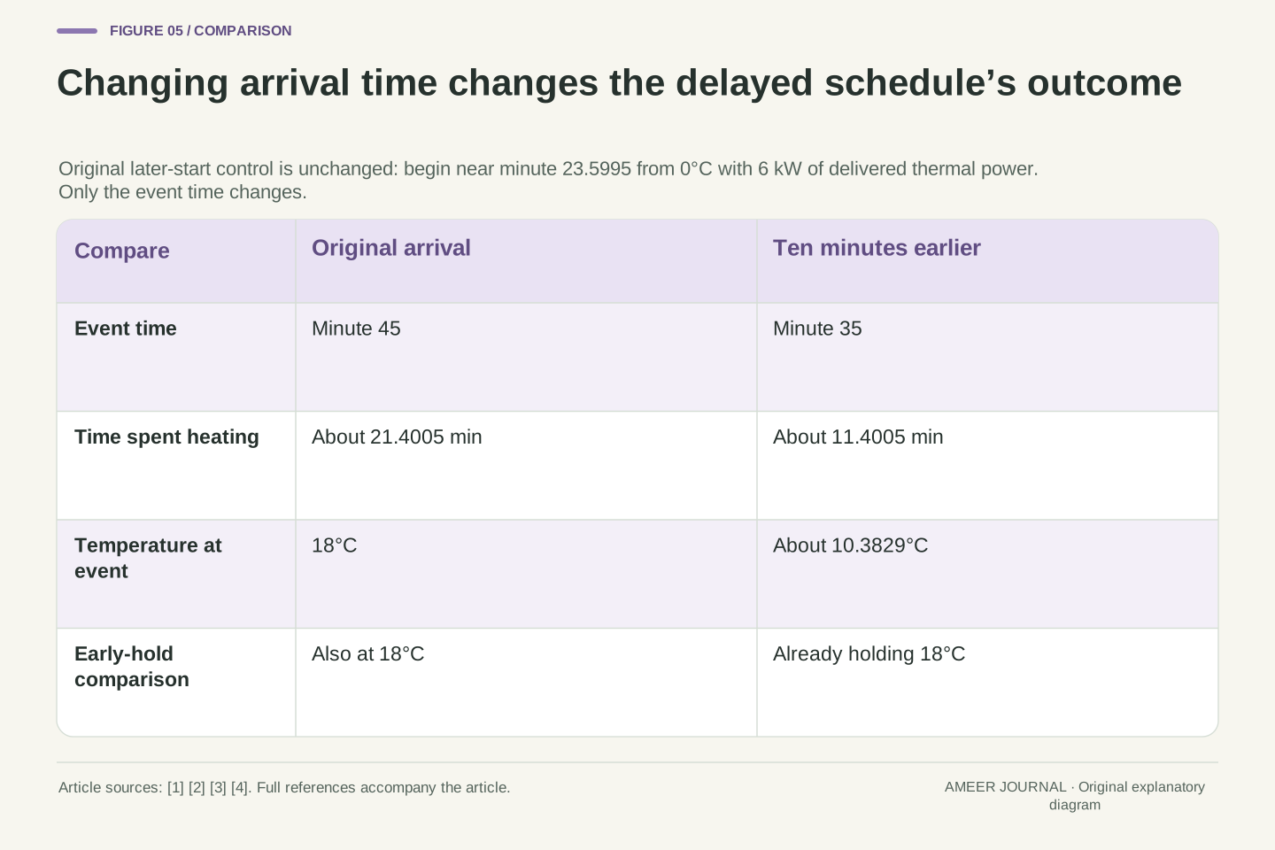
Now keep the third schedule's planned start, but move actual arrival ten minutes earlier, to minute 35. The heater has then run for only about 11.4005 minutes. The calculated arrival temperature is approximately 10.3829°C, well below the 18°C target. The early-hold schedule would already be at 18°C at that time, because its initial warm-up finished before minute 35.

This exposes a trade-off within the model. Waiting avoided heat loss when the event happened exactly on time. Heating early and holding provided a longer interval during which the target was available. No probability of delay or early arrival has been assigned, so these cases do not identify which trade-off a real driver or controller should choose.

Change a different input instead: begin a separate case with the body already at 10°C. Under the same 0°C surroundings and 6-kW heating, reaching 18°C takes about 10.4612 minutes. It requires a smaller stored increase of 0.8 kWh. Outside temperature alone therefore does not describe the starting condition; the body's existing state matters too. The manuals describe preparation as dependent on operating conditions. [1][2]

For the unchanged delayed-start control, replace t_a=0.75 h with t'_a=7/12 h. The active heating duration is t'_a−t_s=0.1900082773 h. Substitution gives θ(t'_a)=10.3828626596 K. Schedule A is already on its hold interval and remains at 18 K. This is a deterministic event-time change, not a statistical forecast or a newly optimized schedule.

A separate initial-state case sets θ₀=10 K. The first-passage time becomes τ ln[(P/G−θ₀)/(P/G−θ*)]=ln(25/21) h=10.46120323 min. Delivered heat is 1.0461203229 kWh, while ΔU=C(18−10)=0.8 kWh. The difference is outward transfer during this shorter warm-up. Initial stored heat is a given boundary condition, not energy created for free by the schedule.

Arrival time and initial state enter different parts of the calculation. The former chooses when the trajectory is evaluated; the latter changes the trajectory itself. Recognizing both helps interpret condition-dependent preparation described in the manuals. [1][2] A useful timing estimate must say which state it assumes now and which future event it is trying to meet.

Suppose delivered heating power is only 1.8 kW from the cold start. That equals the heat leak at the target, but the body approaches 18°C more and more slowly. It never reaches exactly 18°C in a finite time within this ideal model. At minute 45 it is only about 9.4974°C. Being able to maintain a temperature is different from being able to reach it from below by a deadline.

Raise the input to 2 kW. The eventual limiting temperature becomes 20°C, so the 18°C target is now reachable in finite time. However, the calculation requires about 138.155 minutes, much longer than the available 45. At minute 45 the temperature is approximately 10.5527°C. A target can be reachable eventually while remaining infeasible for the chosen event.

The general reason is visible in the heat account: warming slows as outgoing heat approaches incoming heat. [3][4] Real controls may also decline to run under particular conditions; the Hyundai page, for example, names equipment and charge-state restrictions. [2] A requested preparation time cannot by itself establish that the required heating power is available.

At fixed constant P, the equilibrium rise is θ∞=P/G. Setting P=1.8 kW gives θ∞=18 K. From θ₀=0, θ(t)=18 K[1−exp(−t/τ)] remains strictly below 18 K for every finite t. At 0.75 h it equals 9.4974020507 K. Equality of hold power and target loss supplies an equilibrium condition, not finite-time reachability from a colder initial state.

For P=2 kW, θ∞=20 K and the target is below equilibrium. Solving 18=20[1−exp(−t/(1 h))] gives t=ln(10) h=138.1551056 min. At the original deadline θ=10.5526689452 K. Finite reachability and deadline feasibility are distinct: this control satisfies the former but fails the latter. [3][4]

If P/G lies below the target, constant input cannot reach it from the stated cold start at all. These are properties of the assigned thermal model. Separately, the cited Hyundai control may be unavailable under stated equipment or operating conditions. [2] A scheduling analysis should establish its available input before treating a start-time request as a guaranteed thermal outcome.

We can now add a separate invented assumption: 80% of the electricity supplied to a heating system becomes heat delivered into our modeled body. The remaining 20% is assigned outside that body. This is not a manufacturer efficiency or a heat-pump performance claim. Divide delivered heat by 0.8 to obtain electrical input under this particular assumption.

The later warm-up's 2.14005 kWh of heat then requires about 2.67506 kWh of electricity. Early heating plus holding requires about 3.56004 kWh. Their electrical-input difference is approximately 0.884981 kWh. These values are larger than the heat inputs because we have explicitly included a separate conversion difference before heat reaches the body.

Where that electricity comes from is another question. The Model S manual discusses connected charging and preparation, while the Hyundai page warns that conditioning consumes energy. [1][2] Neither our thermal calculation nor the fact of a cable connection establishes a universal split between external supply and battery energy. Additional electrical loads and supply limits need their own account.

Introduce the separate constant ratio η=H_delivered/E_electrical=0.8. Assign the conversion difference to energy transferred outside the modeled thermal body. Then E_C=H_C/η=2.6750620795 kWh and E_A=H_A/η=3.5600434557 kWh. Their difference is 0.8849813761 kWh. The 6-kW thermal warm-up would correspond to 7.5 kW electrical input within this added boundary.

For warm-up, the conversion difference is E_C−H_C=0.5350124159 kWh. This is separate from L_w=0.3400496636 kWh, which leaves the body after delivered heat enters it. The wider account therefore reads E_C=0.5350124159+0.3400496636+1.8 kWh, apart from displayed rounding. Assigning both losses to the same term would conceal a boundary error.

The manuals discuss conditioning energy and connected or charge-state-dependent operation in their own contexts. [1][2] External-supply versus battery withdrawal requires another allocation model; wall-side losses, traction and cabin loads are absent here. The assigned η is not a measured efficiency or a heat-pump COP. Comparing electrical totals requires the same included loads and conversion boundary, not simply replacing a thermal label with an electrical one.

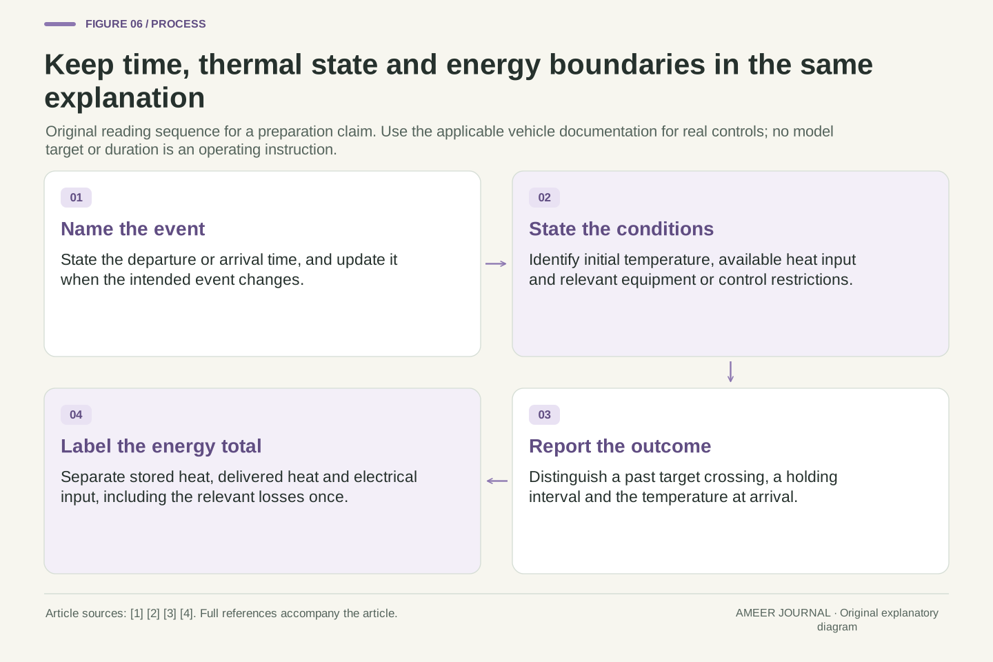
When reading a preparation feature or a result, first find the event it targets. Is the system preparing for departure, for a charging stop, or simply warming immediately? Then look for the starting conditions and any restrictions. The cited manuals discuss scheduling or navigation, thermal conditions, equipment and energy-related limitations; their details belong to the specified vehicle documentation. [1][2]

Next, separate what was reported. 'Reached the temperature' names an earlier event. 'Held the temperature' describes a continuing service. 'Arrived at the temperature' states the condition at the time that matters. Our three schedules show why none of those phrases can substitute for another without knowing the timeline. Also ask whether an energy figure means stored heat, delivered heat or electrical input.

For your own vehicle, use its current documented preparation controls and conditions, and update an arrival or departure plan when it changes. The calculation explains the questions to ask; it supplies no reason to alter hardware or force a particular temperature. A transparent result names its initial state, available input, final state and time, so a reader can tell which benefit the preparation actually established.

A defensible account specifies an event time, initial state, thermal boundary, admissible input and success criterion. State whether success means first passage, maintenance over an interval or a terminal-state requirement. The manufacturer examples show why scheduling and navigation context matter, while their restrictions prevent a generic feature description from establishing universal operation. [1][2]

For comparisons, report both terminal θ and integrated input. Schedules A and C reach 18 K at minute 45 with different heat totals; B has lower input than A but a different terminal state. Earlier arrival reverses the delayed schedule's readiness result without changing its programmed start. Reduced power can turn an otherwise reachable target into a deadline failure. Each conclusion follows from a changed, identified condition.

Finally distinguish thermal preparation from a promised charging rate or whole-trip saving. A thermal target in this model supplies neither a charge curve nor a full vehicle energy budget. Use the appropriate vehicle manual for actual controls and reevaluate the plan when its conditions change. Preserve the input/output boundaries and timing in any reported comparison: they make the result interpretable rather than merely numerically precise.