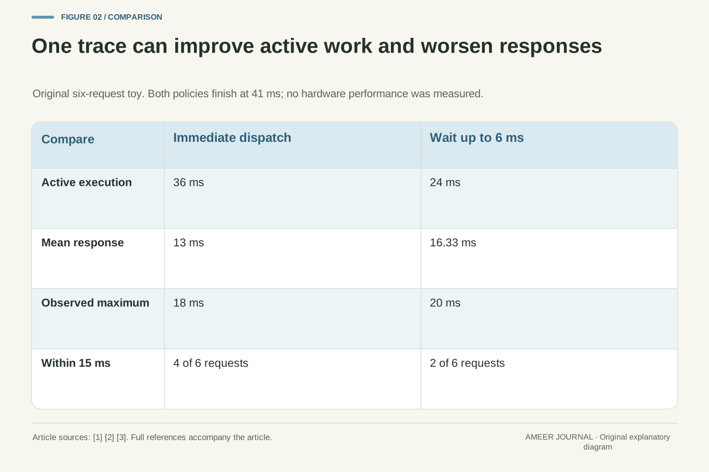
Imagine six small classification requests arriving at an inference service. One setting starts work whenever the machine is free. Another waits briefly so more requests can travel through the model together. In the invented example below, waiting reduces the total time spent processing batches from 36 to 24 milliseconds. Yet the first request receives its answer in 20 milliseconds instead of 8. Both statements can be true because time spent waiting belongs to the reader's experience even when the machine is doing less processing.

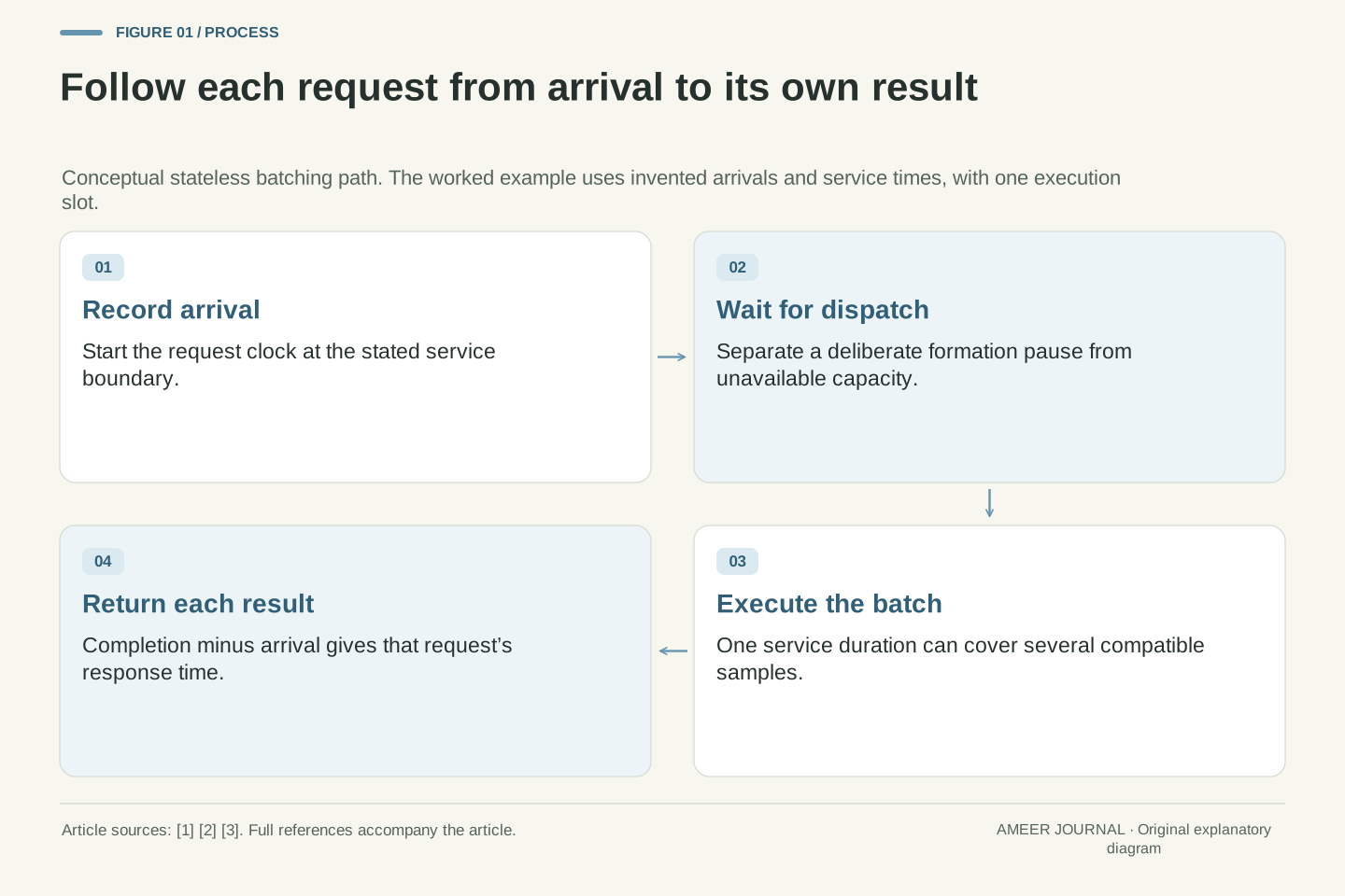
This is the distinction behind dynamic batching. A server collects compatible requests, processes a group and returns the corresponding results. NVIDIA describes its ordinary dynamic batcher for stateless models; Ray Serve describes the queue, batch evaluation and individual responses. [1][2] We will use one fictional stateless model, one execution slot and six precisely timed arrivals. Every timing value is an invented teaching input. The point is to follow the clocks carefully, not to predict the speed of a particular GPU or recommend a setting for an unseen workload. A faster-looking batch counter is only useful when we know which outcome the service needs to improve.

Dynamic request batching combines compatible pending work into a model execution. The scheduling objective is distinct from an individual request's response time. NVIDIA scopes the ordinary dynamic batcher to stateless models, while Ray documents queueing, batched evaluation and distribution of results back to the originating requests. [1][2] These mechanisms make it possible to amortize execution cost, but do not make every latency objective equivalent to throughput or active compute efficiency.

We analyze a deterministic, single-instance, first-in-first-out toy service with six arrivals. The model produces one non-streaming result per input, and every request contains one compatible sample. There is no transport, preprocessing, postprocessing, caching, cancellation, competing model or execution overlap. Durations are stipulated rather than measured. Under those conditions, a six-millisecond formation wait reduces active execution time by one-third while increasing mean response time. Keeping the complete trace visible lets us establish exactly why that happens and where the conclusion stops. The result is a counterexample to an unconditional latency improvement, not a benchmark of Triton, Ray or any model architecture.

Our fictional machine needs six milliseconds of fixed work plus two milliseconds for each item in a batch. A batch containing one item therefore takes 8 milliseconds; two items take 10; three take 12; and four take 14. Four separate one-item batches need 32 milliseconds of active work, while one ready-made four-item batch needs 14. This invented rule captures a possible benefit of sharing fixed work. Real batch costs must be measured for the actual model and hardware; the documentation recommends checking latency and throughput while changing batching settings. [1]

Dividing 14 by four gives 3.5 milliseconds of active work per item. It does not mean each person gets an answer 3.5 milliseconds after submitting a request. In this example, all four results become available when the 14-millisecond execution finishes. A request may also have waited before that execution began. Think of three separate quantities: how long the machine worked, how many items that work covered, and how long each request waited for its result. Dividing the first by the second does not automatically produce the third. That small distinction prevents the most tempting misreading of a batching improvement.

Define the hypothetical service-time function S(b)=6+2b milliseconds for batch cardinality b in {1,2,3,4}. It contains a fixed six-millisecond component and a linear two-millisecond component per sample. Thus S(1)=8, S(2)=10, S(3)=12 and S(4)=14. Four singleton executions consume 32 milliseconds of active service, versus 14 for an already assembled four-item execution. The stipulated curve is neither an empirical fit nor a claim that every model has a linear marginal cost or positive batching benefit.

S(4)/4=3.5 milliseconds is an amortized active-service budget per sample. For simultaneous ready inputs in this non-streaming execution, each completes after S(4)=14 milliseconds, before accounting for any earlier queueing. The quantities have different denominators and measurement boundaries. If a later implementation instead streams or completes members independently, its observable response timing needs a different model. NVIDIA's tuning guidance explicitly considers the tradeoff between latency and throughput [1]. We therefore keep S(b), sample count, dispatch time and completion time separate throughout the trace, rather than calling their different ratios a single speed figure.

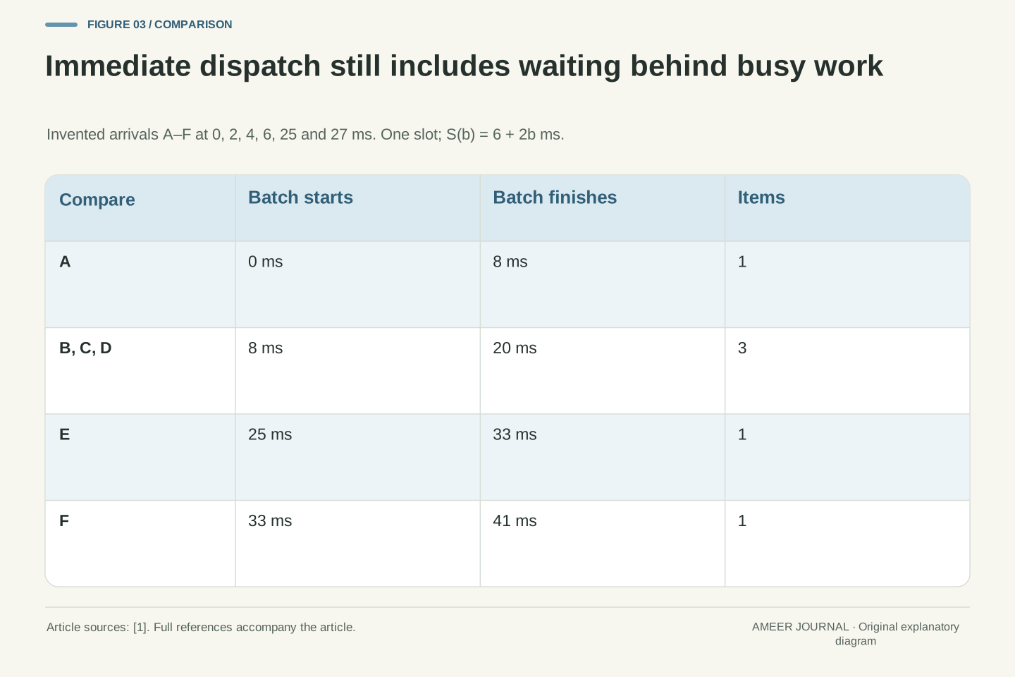
Label the requests A through F. Their arrival times are 0, 2, 4, 6, 25 and 27 milliseconds. The server can place at most four items in one batch. Our first policy starts as soon as the server is free and at least one request is waiting, taking the available requests in arrival order. This resembles the no-extra-delay idea in the documented default dynamic-batching behavior, but the specific arrivals and durations belong entirely to our example. [1] A busy server cannot start another execution until its current one finishes.

A arrives at time 0 and runs alone until time 8. B, C and D have arrived by then, so their three-item batch runs from 8 to 20. E arrives at 25 and runs alone until 33. F arrived at 27 while E was running, so F runs from 33 to 41. Subtract each arrival from its completion: the response times are A 8, B 18, C 16, D 14, E 8 and F 14 milliseconds. There was no deliberate batch-filling pause, yet several requests still waited. That waiting came from an occupied execution slot, which is a different cause from choosing to hold an otherwise ready request for companions.

Let the arrival vector for A–F be a=(0,2,4,6,25,27) milliseconds. The instance is initially idle, capacity is four samples, and the immediate policy dispatches the oldest available compatible samples whenever the instance is free. It introduces no additional formation delay. NVIDIA describes batch construction when a model instance becomes available and documents a default configuration without an intentional formation delay [1]; our simplified dispatcher is explicitly defined rather than inferred to reproduce every backend scheduling detail.

The resulting execution intervals are A:[0,8], BCD:[8,20], E:[25,33] and F:[33,41]. Service durations sum to 8+12+8+8=36 milliseconds. Completion minus arrival gives L=(8,18,16,14,8,14), summing to 78 and averaging 13 milliseconds. B's ten-millisecond queue delay is compatible with a zero intentional formation wait: A is already executing. F similarly waits six milliseconds behind E. The trace establishes a concrete baseline before any parameter changes. Without the arrival vector and instance availability, a list of batch durations alone could not recover these request-level latencies or distinguish capacity backlog from deliberate waiting.

Now change only the formation policy. If fewer than four requests are available, the server may wait until six milliseconds after the oldest waiting request arrived. It starts earlier if four requests become available. When that deadline arrives, it runs the available partial batch. At an exact tie, our example processes the arrival before the dispatch decision. The documented systems also provide size and timeout triggers, but this precise rule defines our toy trace. [1][2] We keep the same model costs, arrivals, maximum size and single execution slot.

A waits at time 0. B arrives at 2, C at 4 and D at 6, filling the batch just as A's waiting limit is reached. ABCD runs from 6 to 20. E arrives at 25 and F at 27; no further requests arrive. At 31, E's six-millisecond limit expires, so EF runs from 31 to 41. The six response times are now 20, 18, 16, 14, 16 and 14 milliseconds. Active processing takes only 14+10=24 milliseconds. A and E paid more waiting time; the other four response times happen to be unchanged. The trace makes those individual outcomes visible instead of hiding them inside the larger batch sizes.

Define a second dispatcher with maximum cardinality four and a formation deadline of oldest_pending_arrival+6 milliseconds. While the instance is free, it dispatches when capacity is reached or that deadline expires; an already expired deadline causes immediate dispatch of available work. Arrival events precede dispatch at an equal timestamp. This explicit model is inspired by the documented maximum-size and timeout behavior [1][2], but is not an assertion about every internal timer transition in those implementations.

At t=6, the queued set {A,B,C,D} reaches four and executes until t=20. At t=25, E opens the next waiting group; F joins at 27. The oldest-arrival deadline is 31, when the two-item group dispatches and finishes at 41. L=(20,18,16,14,16,14), with sum 98 and mean 98/6, approximately 16.333 milliseconds. Active execution is S(4)+S(2)=24 milliseconds. Comparing the traces request by request shows increases only for A and E. This is a workload-dependent outcome, not a monotonic law that every longer wait increases every member's latency or that every larger batch improves completion time. The exact arrival pattern matters to which fixed execution costs are avoided.

The waiting policy cuts active processing from 36 to 24 milliseconds, a reduction of one-third. However, both policies finish all six requests at time 41. If we count completed requests over the same interval from 0 through 41 milliseconds, both give about 146.3 requests per second for this tiny trace. That rate is a description of the chosen finite interval, not a long-running service-capacity measurement. Dividing six by active processing time instead would answer a different question because it leaves out the idle and waiting portions of that interval.

Suppose our invented service target is to finish a request within 15 milliseconds of its arrival. Immediate dispatch meets that target for A, D, E and F: four of six. The six-millisecond wait meets it only for D and F: two of six. Mean latency also rises from 13 to about 16.3 milliseconds, and the largest observed latency rises from 18 to 20. A setting can therefore save active processing work while doing worse against the chosen response target. Documentation advises considering the total latency budget when selecting a wait. [1][2] Six constructed observations explain the mechanism; they do not establish a reliable real-world tail-latency estimate.

Use identical observation boundaries before comparing rates. The six completions over [0,41] milliseconds correspond to 6/0.041, approximately 146.34 completed requests per second, under either policy. The active-service totals differ, but they do not change this finite-window completion rate. A ratio using only busy time would be a service-efficiency quantity with a different denominator. Neither value estimates steady-state capacity without a suitable workload and measurement design. Triton's documentation separates request handling and execution timing, reinforcing the need to preserve those boundaries [3].

For a declared per-request target L<=15 milliseconds, the immediate trace succeeds on four of six requests, whereas the waiting trace succeeds on two of six. Mean latency changes from 13 to 16.333 milliseconds and observed maximum from 18 to 20. The 33.333-percent reduction in active time is therefore insufficient to select the second policy for that objective. NVIDIA recommends measuring the latency-throughput tradeoff, and Ray's guidance places formation waiting within the end-to-end latency budget [1][2]. Do not label our six values p95 or p99 evidence without a defined estimator and meaningful sampling population; here they are exact outcomes of a small deterministic example.

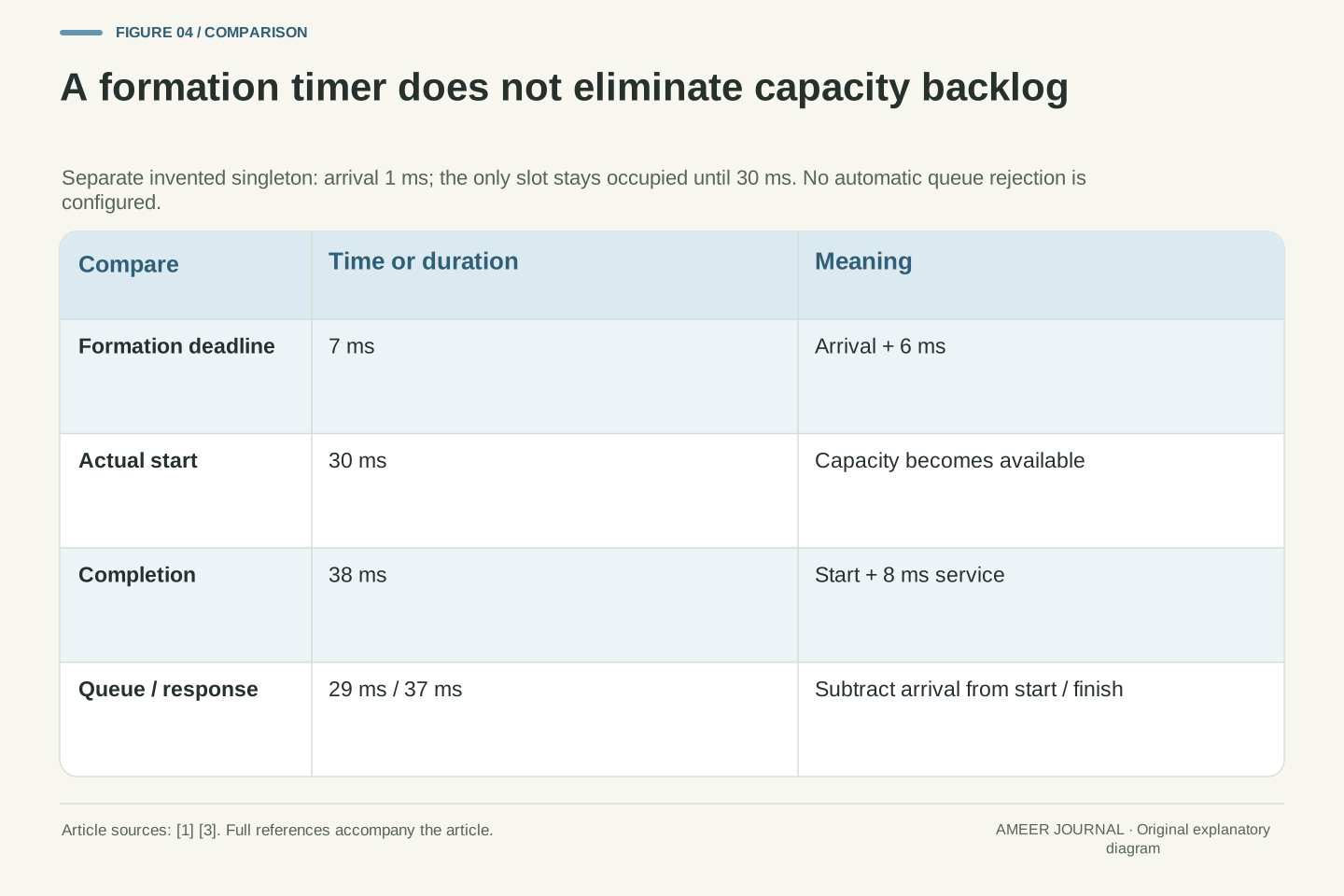
Consider a separate case. The only execution slot is already occupied until time 30. A new request arrives at time 1. Its six-millisecond formation deadline would be time 7, but the slot is still busy. Under our stated scheduling rule, the request starts when the slot becomes available at 30, runs alone for 8 milliseconds and finishes at 38. Its queue wait is 29 milliseconds and its full response time is 37. The batch-filling allowance did not create a six-millisecond response guarantee, nor did it make another execution slot appear.

This is why settings with similar-looking time units need their names and purposes kept together. A deliberate pause to collect companions, a queue timeout that rejects or defers work, and a customer's total response target are different controls. Triton documents queue policies separately from delayed batching and describes requests remaining pending while execution capacity is occupied. [1][3] In a quiet period with no companions, our idle server would simply add six milliseconds before the same singleton execution. The useful question is whether the wait actually forms a beneficial group under the observed traffic, and whether the complete path still fits the service's intended response budget.

Separate deliberate formation delay from capacity queueing. In a second constructed case, the sole instance is unavailable until t=30 and a singleton arrives at t=1. Its oldest-arrival-plus-six deadline is t=7. Once capacity becomes available at 30, the expired deadline permits immediate dispatch; completion is 38. Queue time is 30-1=29 milliseconds and response time is 38-1=37. A bound on an intentional formation wait is not a bound on total time before execution or completion when capacity is unavailable.

This distinction is supported by Triton's description of construction when an instance is available, separately configurable queue-timeout actions, and pending work behind executing requests [1][3]. Frontend work before a request reaches the measured core can also lie outside a particular pending-time metric [3]. Our arithmetic deliberately excludes that work rather than assuming it vanishes in a deployment. Even with an idle instance, a lone arrival under the six-millisecond policy takes 6+8=14 milliseconds instead of 8, because no second sample arrives to amortize the fixed component. A timeout value should therefore be interpreted within its actual scheduler and measurement boundary, not as a standalone latency promise.

Batch size can count requests while missing what those requests contain. Consider a separate text example with four already-tokenized input lengths: 8, 8, 32 and 32 positions. If we store all four in a rectangle padded to the longest length, the rectangle has four rows of 32, or 128 positions. Only 80 positions contain the original input tokens; the other 48 are padding. Hugging Face's versioned documentation describes longest-sequence padding and distinguishes it from truncation, which removes tokens. [4] These counts describe the chosen representation, not a measured runtime.

Grouping the two short inputs together uses 16 positions. Grouping the two long inputs together uses 64, for a total of 80. That is 37.5 percent fewer represented positions than 128, while preserving all 80 input tokens. It does not prove a 37.5-percent speedup: there are now two executions, and their setup costs, kernels and scheduling can differ. Waiting for similarly sized inputs may also add latency. Ray supports defining an effective batch size using item properties rather than only the number of items. [2] The lesson is to record what the limit counts and how the inputs become tensors before interpreting a number such as batch size four.

For already-tokenized lengths (8,8,32,32), longest-sequence padding produces a [4,32] token-ID rectangle with 128 positions. The useful-token total is 80 and padding contributes 48, or 37.5 percent of represented positions. Splitting into length-homogeneous groups produces [2,8] and [2,32], totaling 16+64=80 positions. All original tokens remain; this is regrouping rather than truncation. Transformers v4.49.0 documents the distinction between padding and token-removal policies [4]. The arithmetic counts token positions, not floating-point operations, attention complexity, memory allocation or elapsed time.

Two smaller executions may incur different launch overheads or kernel behavior, and an online length-bucketing strategy can wait longer for compatible partners. Thus the 37.5-percent position reduction is not a proportional performance guarantee. Ray's documented custom batch-size function is an example of measuring capacity by properties of items instead of list cardinality [2]. A token budget must still use the intended tokenizer and representation; counting whitespace-separated words is not generally a model-token count. State whether a cap applies to requests, samples, actual tokens, padded positions or another workload measure before comparing configurations. The limit's unit is part of the experiment, not an incidental label.

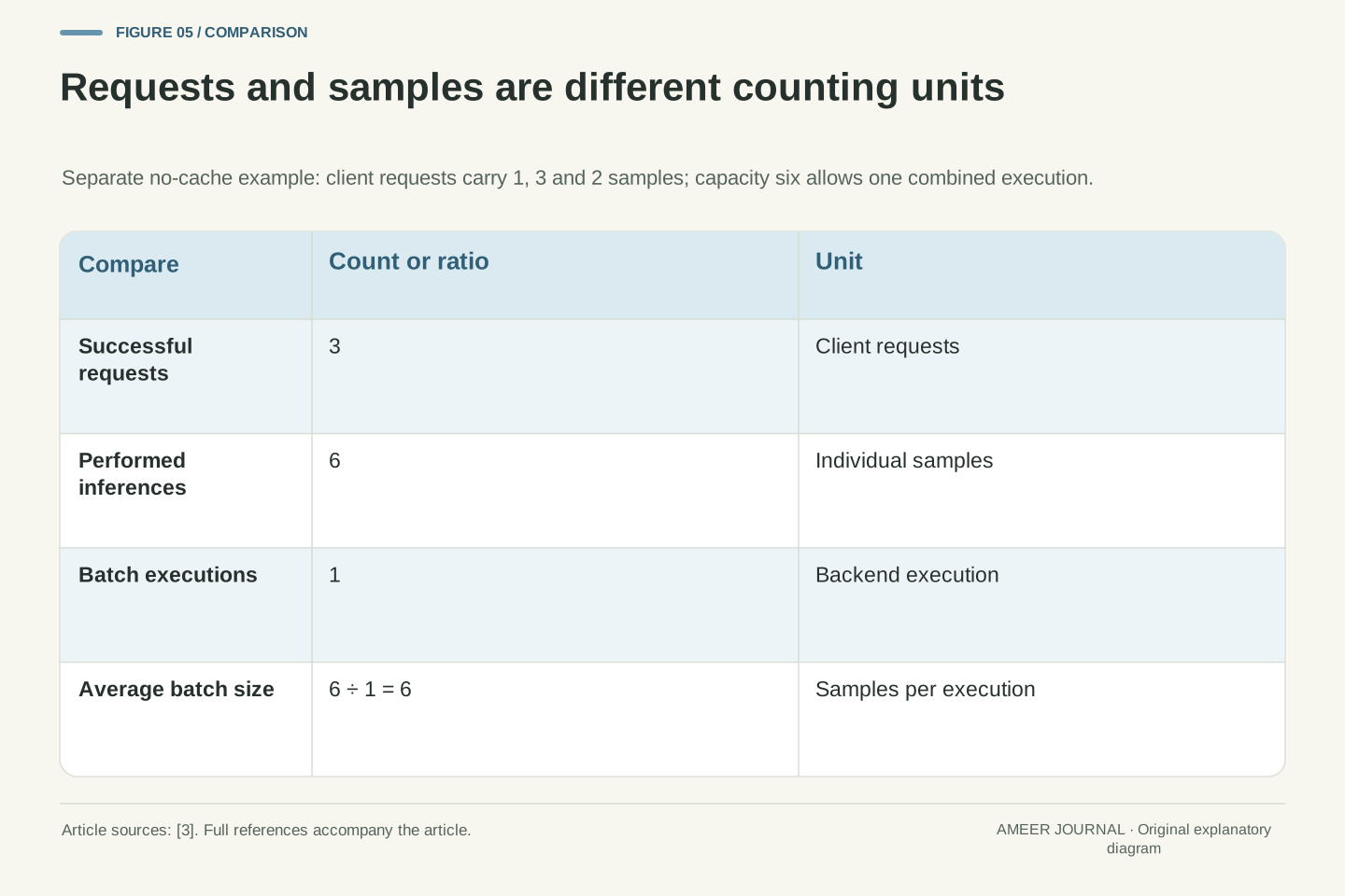
One network request does not always contain one sample. Imagine three successful client requests carrying one, three and two compatible samples. In a separate hypothetical execution with enough batch capacity, the server combines all six samples into one model run. The counts are three requests, six individual inferences and one execution. Calling all three numbers batches would make the dashboard impossible to interpret. Triton's metric documentation explicitly distinguishes these units and describes average executed batch size as inference count divided by execution count. [3]

For this example, the average executed size is six divided by one, or six samples. Three requests divided by one execution would instead describe requests per execution. Both ratios can be calculated, but they answer different questions because client requests can already contain groups. Use matching time intervals and the same model when comparing counter changes. Also preserve whether requests were served from a response cache: the documented inference and execution counters exclude cached requests, while successful-request counts can include them. [3] A changing ratio may reflect a different request mix or cache behavior, so it cannot by itself prove that a scheduler started grouping the same workload more effectively.

Consider three compatible, uncached, successful client requests with sample counts (1,3,2). Suppose a separately configured instance supports six samples and executes all of them together. The increments are request count=3, inference count=6 and execution count=1. Triton's documented semantics distinguish each incoming request, each performed inference sample and each backend batch execution [3]. This example uses different capacity from the earlier four-sample timing trace and does not silently fit six samples into that earlier limit.

The executed mean batch size for an aligned interval is delta(inference count)/delta(execution count), provided the denominator is positive and the scope is compatible. Here it is six. Delta(request count)/delta(execution count) is three, a different statistic because requests can contain their own batches. Counter resets, model/version labels and observation windows need consistent treatment before interpreting either ratio. Cached requests complicate comparisons: the cited inference and execution counts exclude them [3]. Our example stipulates no cache hits so that its bookkeeping is exact. These distinctions help determine whether an apparent improvement came from server-side aggregation, changed client grouping or avoiding inference altogether, rather than treating every higher requests-per-second number as the same mechanism.

So far, each batch ran once and returned complete classification results. Generating text can involve repeated steps, and different requests can need different numbers of steps. A fixed group that stays together until its longest member finishes may leave opportunities unused when shorter members finish earlier. Triton's documentation describes continuous or inflight batching as forming groups at individual iteration steps, allowing newly available slots to be reused. [1] That is a different scheduling mechanism from merely waiting a few milliseconds before starting one complete model call.

The difference matters when reading a performance claim. A service might change the initial waiting policy, the number of concurrent executions, the way unfinished sequences are scheduled, or several of these at once. Those changes should not all be credited to one larger batch number. In our six-request example, no request generates a sequence and no slot is refilled during an execution. The example therefore cannot predict token-generation throughput or first-token delay. For a real service, keep a request's identity attached to its outputs throughout grouping and splitting. Ray's ordinary batched-method contract requires a corresponding result for each input. [2] Efficient grouping still has to return the right result to the right caller.

The timing model covers non-streaming, one-shot stateless inference. Autoregressive serving adds repeated iterations and variable completion lengths. Triton's documentation distinguishes ordinary dynamic batching from stateful sequence batching and describes iteration-level inflight batching that releases completed requests and combines new work with unfinished work at a subsequent step [1]. Its iterative-sequence support is explicitly provisional and backend-dependent, so that documentation is not a guarantee that every deployed model can enable identical behavior.

Changing batch membership between decoding steps is distinct from delaying initial dispatch to collect a larger static group. Comparing those mechanisms also requires identifying whether latency means first response, inter-token timing or final completion. None is measured by our constructed classification trace. Request-to-output correspondence remains a correctness condition across scheduling changes: Ray requires the ordinary batched method's output list to match its input-list length so individual responses can be distributed appropriately [2]. A useful evaluation records the actual scheduler, model mode and output boundary before attributing any result to batching. This avoids extrapolating a simple fixed-cost saving into claims about sequence state, memory management or generation quality that the example never evaluated.

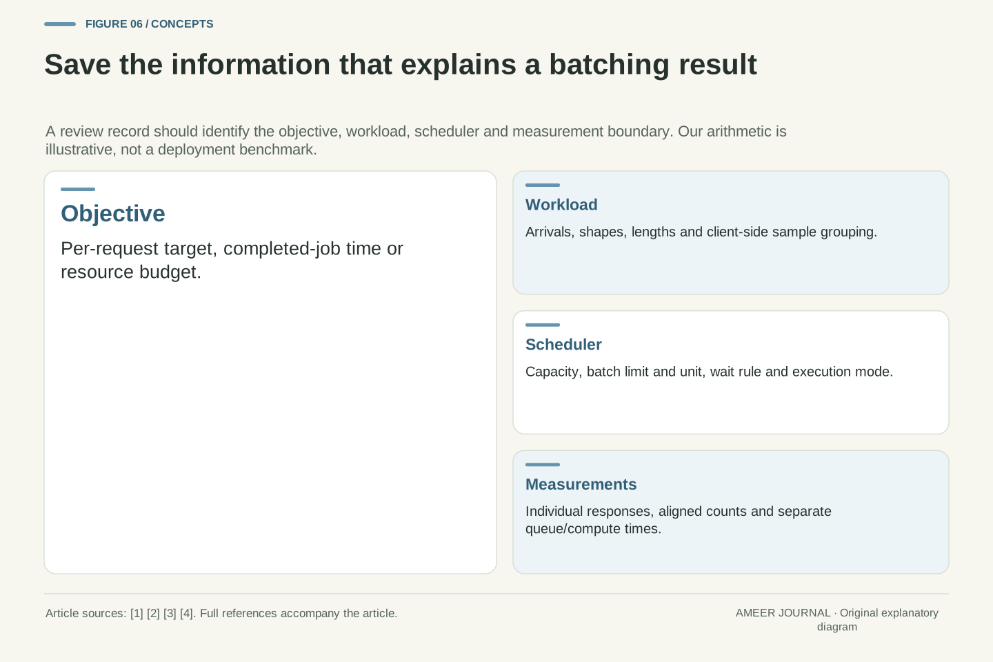
Start a batching comparison with the question the service must answer. Is the priority a response target for each request, completing a large offline job, or processing more samples within a resource budget? Then save the arrival pattern, input shapes, model version, execution capacity, grouping rules and the timing boundary. Measure individual completion times as well as total completed work. The documented tuning guidance and separate queue, input, compute and output metrics provide useful pieces of that record. [1][2][3] They help explain a result instead of leaving only a before-and-after batch-size label.

Our example ends with a clear choice under its stated 15-millisecond target: immediate dispatch meets the target for more of these six requests, even though the waiting policy uses less active processing. Another arrival pattern, service-time curve or objective could favor the waiting policy. The useful result is the method of comparison: subtract arrival from completion, keep the observation interval fixed, count the correct units and inspect who waits. When someone presents an improvement, those details show whether it is a real benefit for the intended service or simply a better number for a different question. They also identify what must be measured next before changing a production configuration.

Define the objective and preserve a reproducible workload before optimizing a batch parameter. Record arrival timestamps, sample shapes and lengths, client-side grouping, maximum size and its unit, intentional waiting policy, instance concurrency, scheduler mode and model/runtime revision. Collect per-request latency alongside aligned completed-work rates and execution counts. NVIDIA and Ray both describe performance tuning in relation to latency, while Triton separates scheduling, input, inference and output durations [1][2][3]. These observations support causal interpretation more directly than a lone utilization percentage.

For the specified six-request trace and L<=15-millisecond objective, immediate dispatch attains four successes versus two for the waiting policy. The latter saves one-third of active service time but has the same final completion timestamp and worse mean latency. Those statements are exact analytical results under the written assumptions. They neither identify a universally optimal wait nor estimate an unseen deployment's capacity. Changing traffic burstiness, service cost, batching compatibility or concurrency requires a new trace or measurement. Preserve both the configuration and the observed boundary so a future comparison can tell whether a gain came from amortized work, changed queueing, altered input representation or a different counting convention.