What you’ll take away
- An ordering test needs both an appropriate data-order assumption and a fixed measurement.
- An inclusive exact tail includes the observed order and equal scores.
- Randomized tail counting has a finite resolution set by its declared number of draws.
- False-positive rate, exposure among flags and an observed p-value condition on different events.
- A negative ordering finding leaves other forms of exposure open.
What does the test actually ask?
Imagine a model scores unusually well on a public benchmark. One possible explanation is that some benchmark material appeared in its training data. But a high task score alone does not tell us what the model saw. Researchers have proposed another clue: compare how likely the model finds the benchmark's original order with how likely it finds shuffled orders of the same examples. Oren and colleagues study this approach using access to sequence log probabilities. [1] Their question is about a particular statistical signal in the ordering, not simply whether the model answers correctly.
The result can include a p-value. A small number is easy to turn into a stronger claim than the analysis supports: for example, saying that p=0.01 means there is a 99% chance the model saw the benchmark. That reverses the conditioning. The American Statistical Association explicitly distinguishes a p-value from the probability that a hypothesis is true. [3] We will work through a small ordering example, then a separate screening example, to make the difference visible. All numbers in those examples are stipulated or calculated here. They are not measurements of any commercial model. The useful outcome is a way to read a contamination report without losing its assumptions or treating a single number as a complete training history.
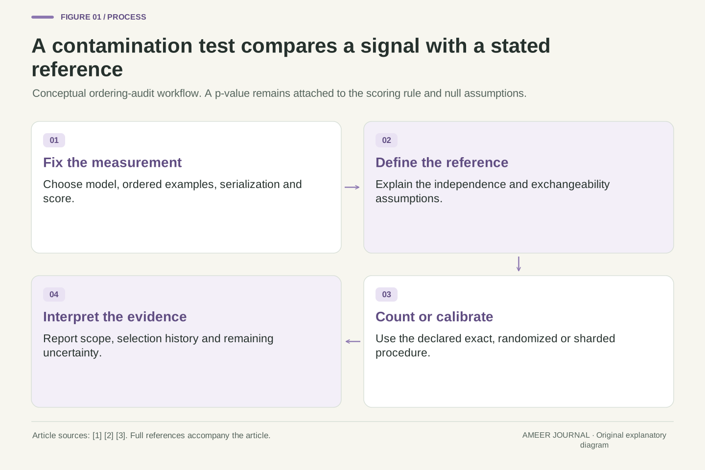
An ordering-based contamination audit compares a benchmark's canonical serialization with serializations formed by permuting its examples. Oren et al. formulate a test using a target model's sequence log-probability queries, with a null in which the model and benchmark are independent [1]. The motivation is that exposure to an ordered benchmark may leave an ordering-sensitive likelihood signal. This is a different observation from the model's benchmark accuracy and does not by itself estimate the resulting score inflation.
A p-value evaluates the extremeness of a statistic relative to a specified null reference procedure. It is not P(contamination|observed result), nor does one minus the p-value supply that posterior probability [3]. We develop an exact finite ordering construction, a randomized-tail calculation, and a separate conditional-count example. The score table and screening rates are declared analytical assumptions; no likelihood API or trained model is queried. This separation makes it possible to verify the arithmetic while keeping the research mechanism distinct from a real audit. It also prevents a small p-value from silently becoming a claim about which benchmark items were copied, when the copying occurred, or how much their exposure changed downstream task performance. Those are additional questions requiring additional evidence.
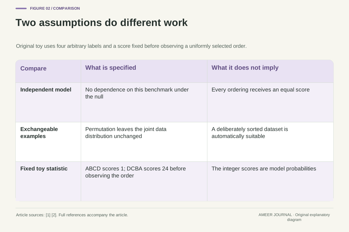
An interchangeable order is an assumption about how data arose
The ordering comparison needs a reason why shuffled orders provide a fair reference. In the paper, that reason is exchangeability: under the relevant data-generating process, changing the order does not change the joint distribution of the examples. The null also assumes the model is independent of the benchmark. [1] These are two different requirements. A model may be independent of a newly collected dataset while still preferring the way that dataset was deliberately sorted.
For our toy calculation, give four distinct items the arbitrary labels A, B, C and D. Before choosing the observed order, fix a scoring rule: list the 24 orders alphabetically and assign scores 1 through 24 in that order. ABCD receives 1 and DCBA receives 24. These numbers are just fixed ordering scores, not probabilities. Under our toy null, choose the observed order uniformly from all 24 possibilities. The scoring rule stays fixed throughout. It would be invalid to look at the observed order first and then define the score to reward matching that same order. That would manufacture an unusually high score by construction. The distinction is practical: keep the model, serialization and scoring choices fixed before interpreting how surprising the observed ranking is.
The paper's permutation argument combines exchangeability of X with independence of the target model from X under the null [1]. Exchangeability is an invariance of the joint data distribution under permutations. It does not assert that a fixed model assigns identical scores to every ordering of one realized dataset. Order-specific preferences may remain; the reference argument concerns how the observed ordering is distributed relative to those preferences.
Our explicit construction conditions on four distinct arbitrary labels. Let Ω contain their 4!=24 permutations. Define a deterministic statistic T by assigning each ordering its one-based lexicographic rank before observing the canonical order. Thus T(ABCD)=1 and T(DCBA)=24. Under the stipulated null, the canonical ordering is uniform on Ω, independent of any adaptation of T. This construction intentionally uses scores rather than invented model likelihoods. A statistic defined after seeing the canonical order as similarity to that order would violate the fixed-before-observation setup: the observed object would always receive a privileged score. The same concern motivates preserving an audit's scoring and formatting choices before inspecting results. Without the relevant invariance, a permutation calculation may be computable while lacking the interpretation that its null reference was meant to provide.
Count the observed order as part of the exact comparison
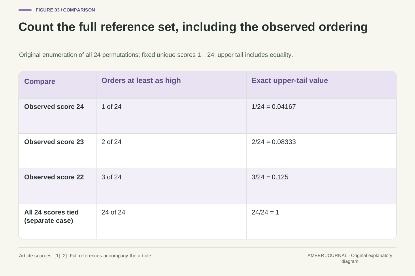
Suppose the observed order in our toy is DCBA, with score 24. We compare its score with every one of the 24 possible orders. Our one-sided rule counts scores at least as large as the observed score. Only DCBA qualifies, so the exact tail proportion is 1/24, approximately 0.04167. The observed order belongs in the comparison. Removing it and reporting zero would answer a different question. SciPy's documented upper-tail convention similarly includes values equal to the observed statistic. [2]
If the observed order instead has score 22, then scores 22, 23 and 24 qualify. The proportion becomes 3/24=0.125. The same scoring rule and reference set now produce a less extreme result. Neither number says what fraction of model training examples were contaminated. They describe positions in this particular ordering comparison. There are only 24 possibilities, so the smallest attainable exact value here is 1/24. Repeating the arithmetic more often cannot create a smaller exact tail for this same finite setup. A larger benchmark may have many more possible orderings, but the resulting calculation must still specify what was shuffled, which direction was counted, and whether the full set or a random sample was used.
Use the inclusive upper-tail statistic p_exact(x)=#{ω in Ω:T(ω)≥T(x)}/24. The direction is declared in advance: higher scores are the candidate signal. For x=DCBA, T(x)=24, and the numerator is one, giving p_exact=1/24≈0.041667. For the ordering with T(x)=22, the numerator is three and p_exact=3/24=0.125. These are exact counts over the complete group, including the observed ordering once. We use the inclusive convention documented for a greater-tail test in SciPy [2], rather than presenting the toy as a literal transcription of the paper's equations.
The finite reference set determines the resolution. With distinct scores, attainable p-values are 1/24,2/24,…,24/24. Adding one again to the exact numerator and denominator would unnecessarily alter this already complete enumeration; the randomized plus-one calculation discussed later has a different accounting boundary. The score units themselves are irrelevant to these ranks: replacing scores 1…24 with any strictly increasing transformation preserves every tail count. That invariance is another reason not to interpret the numerical p-value as a magnitude of model memorization. Its value summarizes the ordering statistic relative to a reference distribution, not an exposure fraction, a copied-token count or a change in task accuracy.
A five-percent rule describes repeated null cases
Now imagine repeating our toy experiment under its null. Each time, choose the observed order uniformly from the 24 possibilities and use the same fixed scores. Adopt the rule “flag when p is at most 0.05.” Only the order with score 24 is flagged. The next score gives 2/24, about 0.08333, which is above the threshold. Therefore the fraction of null cases flagged is 1/24, about 4.17%. This is below 5% because our possible p-values occur in discrete steps.
That repeated-case statement is not a probability that one flagged case is innocent. It describes how the rule behaves when the stipulated null generates cases. Also notice what happens with ties. If every order receives the same score, every score is at least as large as the observed score. The inclusive tail is then 24/24=1, and nothing is flagged. Finally, deliberately choosing DCBA as the stored order every time would break our uniform-order assumption. Our fixed rule would then flag every case, even without adapting the scorer to the dataset. A correct division cannot rescue an inappropriate reference assumption. Check how the benchmark acquired its order before treating a low value as evidence about training exposure.
Under the toy null, the canonical ordering is uniform on Ω. At the prespecified rejection rule p_exact≤0.05, only the maximum-score ordering rejects because 1/24≤0.05<2/24. Hence P(flag|null)=1/24≈0.041667. The finite grid produces a conservative threshold outcome relative to 0.05. This direct enumeration verifies the false-alarm statement without invoking an asymptotic approximation or fitting a sampling distribution.
Ties change the rank distribution. With T constant on Ω, every inclusive p-value equals one, rather than being uniformly spread across the grid. Counting equality protects the reference comparison from claiming that a tied observation uniquely exceeds all alternatives. The null also matters independently of arithmetic: a data-publishing process that always selects DCBA produces p_exact=1/24 on every release under this fixed scorer. The resulting flag frequency is one, because that process is not the stipulated uniform-order null. This counterexample isolates an exchangeability problem without alleging that the scorer saw any particular release during training. In an actual audit, the relevant question is whether the benchmark's construction and ordering support the proposed permutation reference, not whether software can mechanically generate shuffled copies.
Why zero exceedances does not mean a zero p-value
Enumerating every order soon becomes impractical. A randomized procedure instead samples a declared number of shuffled orders and compares their scores with the observed score. Let m be the number of sampled permutations, and b the number whose scores are at least as large as the observed score. Under the plus-one convention we use, the reported value is (b+1)/(m+1). SciPy documents this adjustment for randomized permutation tests. [2] It includes the observed statistic in the comparison rather than treating a finite sample as every possible outcome.
For a separate example with 99 sampled permutations, suppose none reaches the observed score. Then b=0 and the value is 1/100=0.01, not zero. If four do, it is 5/100=0.05. With 999 sampled permutations and no exceedances, the smallest result is 1/1000=0.001. More samples change the attainable resolution, but do not repair a wrongly chosen null, a changing model, or a score chosen after inspecting the data. These examples concern random samples from an appropriate permutation reference; they are separate from our complete enumeration of 24 orders. Keep the sampling design and random seed with the result so another reader can distinguish a reproducible simulation from a full exact count.
For a randomized upper-tail comparison, declare m independent uniform permutation draws with replacement from the relevant permutation reference and hold the statistic fixed. Let b count sampled scores at least as extreme as T_observed. The conservative convention illustrated here reports p_MC=(b+1)/(m+1), consistent with SciPy's documented randomized-test adjustment [2]. Sampling may revisit an ordering; the counting procedure must match its declared design. This is not an instruction to apply SciPy's default sample-label permutation mode to a benchmark-order audit without configuring the appropriate statistic and transformations.
The arithmetic gives p_MC=0.01 for m=99,b=0 and p_MC=0.05 for m=99,b=4. With m=999,b=0, the floor is 0.001. These floors are consequences of the chosen randomized counting rule. They do not apply to every method that returns a p-value. In particular, the 24-order exact calculation already includes the observed order in its complete reference set and uses its exact tail proportion directly. Preserve the draw count, replacement policy, direction, tie handling and randomness record. For floating-point model scores, also define how numerical ties are recognized; the SciPy documentation explicitly discusses finite-precision comparisons [2]. A sample with no observed exceedances establishes only the reported resolution of that procedure, not the impossibility of an equally extreme null result.
Reverse the conditioning only with additional information
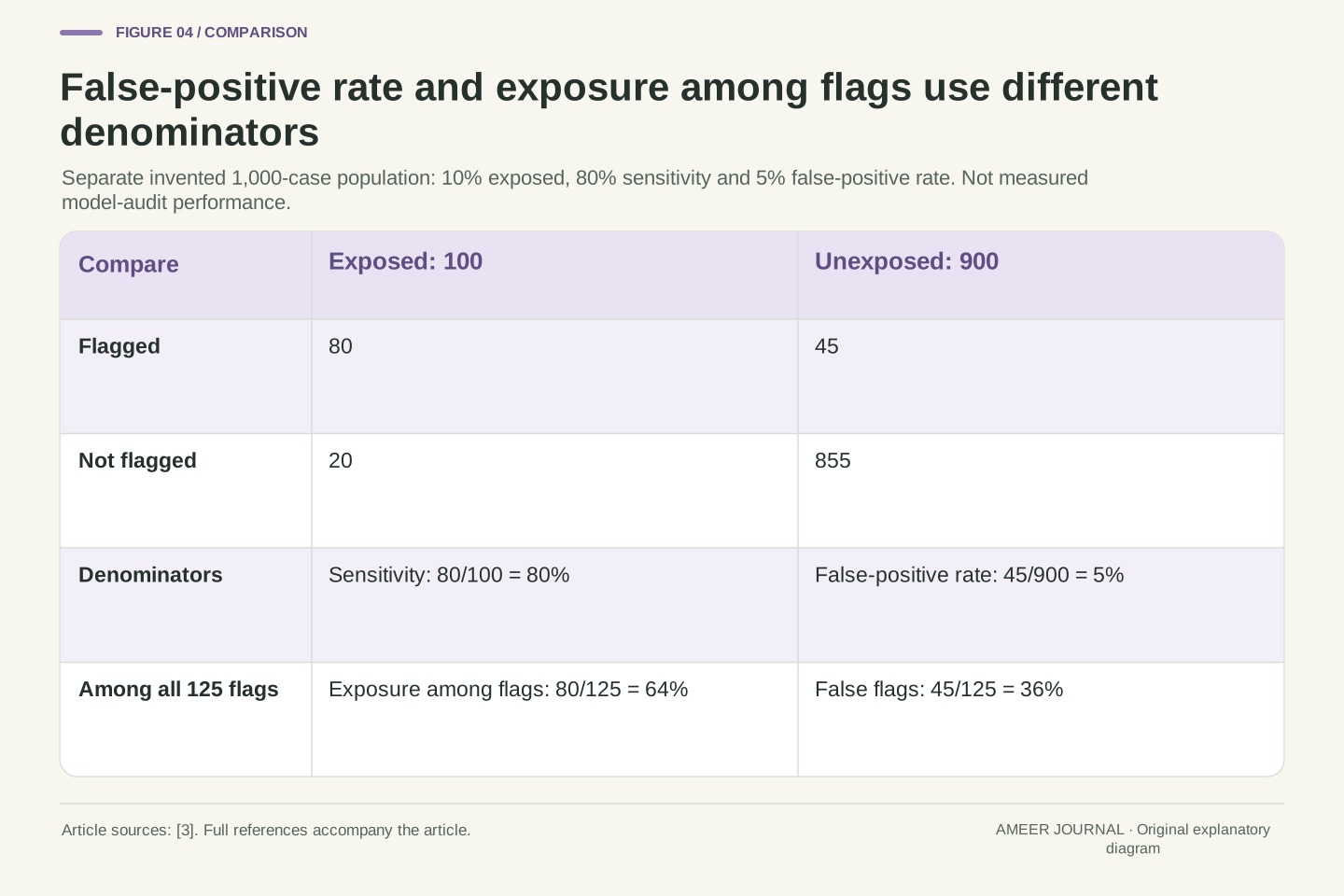
To see why a false-alarm rate is not the fraction of flags that are wrong, use a separate invented screening population. Imagine 1,000 model–benchmark pairs. Suppose 100 were exposed and 900 were not. Assume a particular screening rule flags 80% of exposed pairs and 5% of unexposed pairs. These rates are invented for the example; they are not measured properties of the research method and are not calculated from a p-value.
The rule flags 80 of the 100 exposed pairs. It also flags 45 of the 900 unexposed pairs. There are therefore 125 flags, of which 80 correspond to exposure: 80/125=64%. A 5% false-alarm rate did not produce 95% exposed cases among the flags. The two percentages divide by different groups. If exposure were rarer while the assumed screening rates stayed the same, false flags could make up a larger share of all flags. This does not make screening useless. It shows what extra information is needed to interpret an individual flag: the prevalence of the condition and the rule's behavior in both exposed and unexposed cases. A p-value alone supplies neither of those missing inputs. The example is a counting demonstration, not an estimate of contamination in available models.
Consider a separately stipulated population of 1,000 model–benchmark pairs with exposure prevalence 0.10. Assume sensitivity P(flag|exposed)=0.80 and false-positive rate P(flag|unexposed)=0.05 for one declared screening rule. These inputs describe the rule over populations; they are not inferred from one observed p-value and do not represent measured performance of the cited paper. The expected-count construction contains 100 exposed and 900 unexposed pairs, with 80 true flags and 45 false flags.
Conditioning on the 125 flagged pairs gives P(exposed|flag)=80/(80+45)=0.64 within this invented population. Equivalently, 0.80×0.10 divided by [0.80×0.10+0.05×0.90] equals 0.64. The denominator changes when conditioning changes. A nominal significance threshold, an attained p-value, a sensitivity estimate and a positive predictive value are therefore different quantities. Even this illustrative posterior concerns the coarse event “flag,” not the full information in an exact observed statistic. A richer posterior would require an appropriate probabilistic model and further evidence. The counting example makes no claim that real exposure prevalence is known or that all exposed training histories produce the same detectable ordering signal. Its purpose is to demonstrate why replacing those unknowns with 1−p is an unjustified operation.
A missing ordering signal leaves other exposure routes open
A report may find no unusual preference for the benchmark's stored order. That is a result about the chosen signal under the tested conditions. It does not establish that the model never encountered related material. The paper explicitly limits what its tests can rule out: exposure can occur through material used to build a benchmark, rather than through ingestion of the full test set in its original form. [1] The assumptions needed for reliable detection are different from the assumptions used to control false alarms.
An ordering test is easiest to understand as a question about a particular trace: does the original arrangement receive an unusually favorable score? Other traces could require other investigations. For example, examining known data records, comparing overlap with source documents, or evaluating on newly constructed examples would ask different questions. Those approaches also need their own methods and limitations; listing them does not certify a model as clean. Phrase a negative finding at its actual scope: this procedure did not detect its target signal in this model version and benchmark representation. Preserve the number of items, the ordering, the score definition and the test settings. That record gives later reviewers a clear starting point if new training-data information becomes available.
Non-rejection is not a proof of independence or absence of exposure. The paper separates its null false-positive argument from the additional conditions required for useful power, and its limitations identify partial contamination through benchmark source material as outside what the method can exclude [1]. Thus a null-compatible observed statistic can coexist with training histories that do not create a sufficiently detectable canonical-order preference. This is a scope distinction, not an estimate of how frequently those histories occur.
The practical report should name the detection target and preserve the tested representation. A statement such as “no ordering signal detected by this procedure” is more identifiable than a global claim of uncontaminated training. If another audit later measures document overlap or evaluates on newly assembled questions, its result should remain attached to that separate target and protocol. Combining different kinds of evidence may support a stronger conclusion, but it requires explaining their relationships and assumptions. For this article's fixed-score toy, a large exact p-value merely means that many reference orders receive at least the observed score. It cannot establish the actual data history of a model, because the toy never included a model or a training process. Keeping that boundary visible prevents a successful statistical calculation from being mistaken for a complete provenance audit.
Searching across many tests changes the reporting question
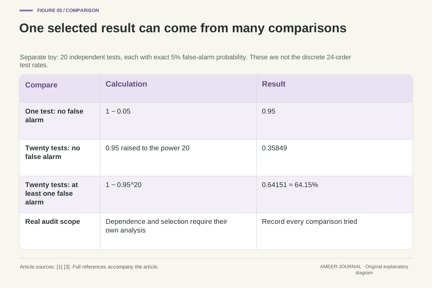
Suppose an analyst tests many benchmarks, serialization choices or model versions, then highlights only the smallest result. The reported number has been selected from a larger search. To illustrate the effect, imagine 20 independent tests, each with exactly a 5% false-alarm probability under its null. The chance of no false alarms is 0.95 multiplied by itself 20 times, about 0.3585. The chance of at least one is therefore about 0.6415, or 64.15%. These assumptions define a new toy example; this is not the false-alarm rate of our discrete 24-order calculation.
Real audit tests may be dependent, so that 64.15% figure cannot simply be copied into a report. Its purpose is to show why the complete family of comparisons matters. Decide which question is primary, record the alternatives tried, and state any adjustment or separate confirmation procedure. The contamination paper itself notes that its reported p-values did not receive multiple-test corrections. [1] That limitation belongs beside the findings when interpreting them. Searching is often part of learning how a method behaves, but a result chosen during exploration should be identified as such. Transparency lets readers distinguish a predeclared comparison from the most striking outcome found after many attempts.
In a separate multiplicity construction, let 20 independent null tests each have an exact rejection probability of 0.05. The family probability of at least one rejection is 1−(1−0.05)^20≈0.641514. Independence and the per-test probability are stipulated. This calculation does not use the 1/24 rejection probability of the earlier exact-order example, and it does not quantify the behavior of correlated real benchmark audits. It isolates how selection from a family changes the event being reported.
Predefine the inferential family and the intended error criterion before attaching confirmatory meaning to a selected result. Record benchmark variants, model versions, serializers, score definitions and directional choices that were inspected. If a procedure uses a multiplicity correction, disclose the family it covers; if results are exploratory, label that status directly. Oren et al. explicitly report the absence of multiple-test corrections among their limitations [1]. The presence of a nominal per-comparison p-value therefore should not be silently recast as a family-wide guarantee. An additional confirmation dataset or independently fixed analysis may answer a different evidential question, but its independence and selection history also require explanation. The essential point is that a reader needs the search process as well as the displayed minimum.
Keep the exact test separate from the paper’s sharded method
The paper also presents a method that divides the dataset into shards. Within each shard, it compares the original ordering's log probability with an average from shuffled orderings, then combines the shard differences using a one-sided t-test. Its guarantee is described as asymptotic and uses additional assumptions, including independent identically distributed examples. [1] That is a different procedure from counting all 24 orders in our small example.
This distinction matters when reading a very small reported p-value. The minimum 1/(m+1) discussed earlier belongs to the randomized rank-counting rule we specified. It is not a universal minimum for every statistical method. Similarly, a result from a t-test should not inherit the exact finite enumeration argument just because both procedures shuffle data. Start by identifying the actual algorithm. The paper's audit setting also requires sequence log-probability access. [1] A chat interface that only returns generated text does not automatically provide that measurement. Before attempting replication, establish which scores the interface supplies, how the sequence is serialized, and whether the model version is fixed. A fluent answer about its own training data would be a different kind of response, not the ordering-likelihood measurement defined by this test.
The sharded procedure is methodologically separate from our finite permutation enumeration. It forms per-shard differences between canonical log likelihood and an average over shuffled log likelihoods, then applies a one-sided t-test to the collection. The paper characterizes its false-positive validity as asymptotic, with additional i.i.d. and finite-moment assumptions [1]. We do not reproduce its theorem notation as a deployment recipe or assert that an arbitrary finite shard count delivers an exact guarantee.
Consequently, neither the exact 24-order grid nor the randomized (b+1)/(m+1) floor should be assigned to that different statistic. Identify the estimator, aggregation and calibration before interpreting its numerical resolution. Also distinguish the required observation channel from the label “black box.” The paper's setting includes sequence log-probability queries [1]; it is not restricted merely to reading generated answers from an opaque service. A replication record should specify whether the available interface exposes the needed sequence likelihoods and how any length or context constraints affect the scored serialization. These are measurement-contract questions. They do not disappear because model weights are inaccessible, and they cannot be answered by asking the model to state whether it remembers a benchmark.
Write a result that another reader can reconstruct
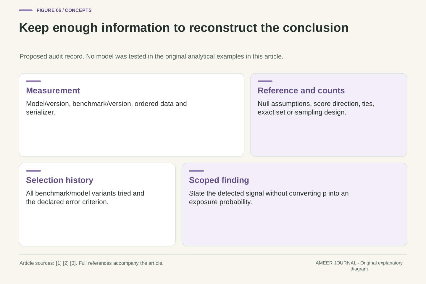
A useful audit record begins with the model version, benchmark version and the exact ordered data representation. Add the score definition, the reason shuffled orders form the chosen reference, the direction of the comparison and the treatment of equal scores. State whether you enumerated all possibilities or sampled permutations. For sampling, preserve the number of draws and the randomness settings. Include the full family of comparisons and explain any exploratory changes. These are proposed record fields drawn from the distinctions we have worked through, rather than a claim that one universal checklist validates every audit.
Our toy report can be precise: with a fixed lexicographic score, a uniformly selected canonical order and all 24 permutations enumerated, observed score 24 has an inclusive upper-tail proportion of 1/24. At a predeclared threshold of 0.05, the rule flags one of the 24 equally likely null orders. That is the result we have actually established. We have not established a 95.83% probability of exposure, identified copied text, or estimated benchmark inflation. Keeping the conclusion attached to the calculation makes the report useful. A later reader can inspect its assumptions, reproduce its counts and decide which additional evidence would be needed for a broader claim about the model's training history.
Preserve the inferential object together with its provenance: target model/version, benchmark/version, ordered examples, serializer, statistic, direction, exchangeability rationale, tie policy and full or sampled reference construction. For randomized analyses, include draw count, replacement design and seed or equivalent randomness record. For a family of comparisons, retain the selection history and calibration rule. These fields are a proposed reproducibility record for the mechanisms discussed here. They do not establish that unobserved assumptions hold or turn one statistical test into a comprehensive training-data investigation.
The precise conclusion of our enumerated construction is conditional: under uniform canonical order over four distinct labels and the pre-fixed lexicographic statistic, observed score 24 yields p_exact=1/24. The p≤0.05 rule has null rejection probability 1/24. For score 22 the exact value is 3/24. All three statements follow from the retained enumeration. None is a posterior contamination probability or a measured effect on model accuracy. A defensible real audit similarly connects its interpretation to the measurement and reference procedure it actually used. Publishing the assumptions and counts allows critique at the appropriate level: the score computation, the data-generation model, the selection process or the scope of the conclusion, instead of debating an isolated p-value detached from its origin.
Sources & further reading
Explore the references behind this guide. External pages may change after our review.
- Proving Test Set Contamination in Black Box Language ModelsOren, Meister, Chatterji, Ladhak and Hashimoto / arXiv · Accessed 6 Nov 2026
- permutation_test — SciPy v1.16.0 ManualSciPy · Accessed 6 Nov 2026
- ASA Releases Statement on Statistical Significance and P-Values, 7 March 2016American Statistical Association · Accessed 6 Nov 2026
Article updated 6 Nov 2026.
Found something we should revisit?
Good explanations get better with thoughtful feedback.