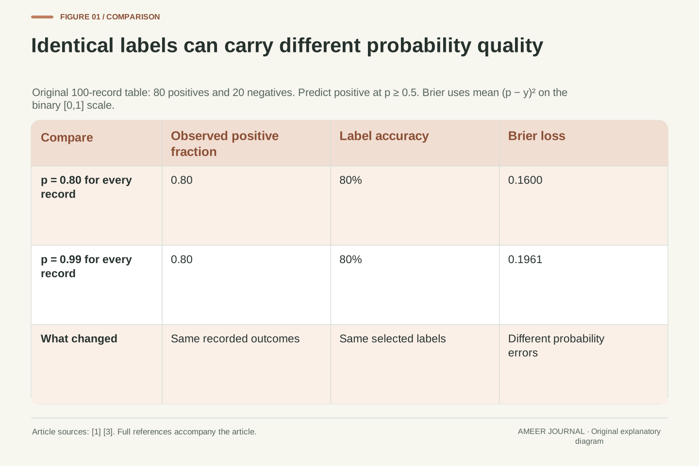
Imagine a program deciding whether a photograph contains a bicycle. We construct one hundred written test records: eighty say a bicycle is present, and twenty say it is absent. These are invented labels for a calculation, not photographs we submitted to a model. One prediction set assigns a 99 percent probability of “bicycle present” to every record. Another assigns 80 percent to every record. With a rule that predicts “present” at probabilities of at least 50 percent, both sets give exactly the same one hundred labels.

Both therefore get eighty labels right. Their accuracy is identical, but the probability statements differ. Among records assigned 80 percent, the constructed positive fraction is also 80 percent. Among records assigned 99 percent, it is still only 80 percent. Calibration concerns this relationship between probability estimates and outcome frequencies. [1] Accuracy alone cannot reveal it.

The distinction matters whenever a reader uses probabilities to compare uncertainty. A correct class label and a well-supported probability are different outputs. We will keep the labels, thresholds and arithmetic visible so that the examples explain the measurement rather than pretending to rank real AI products.

Construct N=100 binary records with eighty y=1 labels and twenty y=0 labels. Let prediction set A assign p=0.99 to every record and set B assign p=0.8. Define the decision rule explicitly as predicted y=1 whenever p≥0.5. Both sets predict the positive class on every record and obtain accuracy 80/100=0.8. No trained classifier or image dataset is involved in this construction.

The empirical probability comparison differs: A's mean predicted positive probability is 0.99 while the observed positive fraction is 0.8; B's corresponding values are both 0.8. Probability calibration asks whether event frequencies agree with assigned probabilities, rather than whether thresholded labels merely match targets [1]. Exact agreement in this finite constructed sample is not proof of population calibration or future performance.

We retain the full stipulated prediction/label tables and independently reproducible arithmetic. This lets us separate threshold accuracy, binary probability scores, binned diagnostics and conditioning on subgroups. Each is a distinct summary of a declared record. In particular, an unchanged accuracy does not imply an unchanged probability assessment, and improved numerical agreement on an inspected sample does not by itself establish an independently validated calibration method.

In these examples, the percentage always means the probability that a bicycle is present. It does not always mean the probability that the program's chosen label is correct. Consider a record assigned 20 percent. Our 50 percent decision rule chooses “bicycle absent”. The model's implied probability for that chosen negative label is 80 percent, because the two classes exhaust the possibilities in our setup.

A positive-class calibration chart must therefore compare the 20 percent value with the proportion of records that actually contain a bicycle. It should not compare that value with the proportion correctly labelled “absent”. The scikit-learn curve documentation explicitly defines its inputs as positive-class probabilities and its observed output as the fraction of positive labels. [2] Mixing these conventions can reverse the interpretation of a perfectly ordinary chart.

Record the positive label, the probability column and the decision rule before calculating anything. If a label is ambiguous or has been recorded incorrectly, a neat chart cannot repair it. The same caution applies when someone writes “I am 90 percent sure” in a chatbot answer: our examples concern defined classifier probabilities paired with binary outcomes, so that sentence needs its own defined evaluation before it can be interpreted in the same way.

Let p denote the probability of the specified positive event Y=1, not an unspecified confidence score. For p=0.2, the declared threshold selects the negative class, whose assigned probability is 1−p=0.8. Positive-class calibration compares p with the conditional positive frequency. Top-label confidence would instead pair the selected class's probability with an indicator of whether that selected label was correct. These are different transformations of the same binary prediction.

The calibration_curve interface documents positive-class probabilities, an explicit positive label and a returned fraction of positives [2]. Our calculations use that convention throughout. We do not replace y with a correctness indicator while leaving p unchanged. Class-column order and the decision threshold therefore belong in the evaluation record alongside the outcome labels.

This distinction also limits the scope of the article. A language model's verbal confidence statement, an unnormalized score and a classifier's defined positive-class probability are not interchangeable data types merely because each can be written as a percentage. Applying a calibration analysis to another output requires defining the event and pairing the score with appropriate outcomes. The arithmetic here does not independently establish the quality of those outcome labels or convert an ambiguous statement into a well-defined probabilistic forecast.

A binary reliability diagram groups predictions and places each group using two numbers: its average predicted probability and its observed fraction of positive labels. Agreement places the point on the diagonal. In our opening example, the 80 percent predictions make a point at (0.8, 0.8). The 99 percent predictions make a point at (0.99, 0.8). Their identical accuracy does not put them in the same place. [1][2]

Keep the number of records behind each point. Eight positives out of ten and eight hundred out of a thousand both produce a fraction of 0.8. Yet changing one positive label to negative moves the first fraction to 0.7 and the second to 0.799. The first change is ten percentage points; the second is one tenth of a percentage point. These exact arithmetic changes illustrate why a plotted fraction without its count leaves out useful information.

They are not confidence intervals. The relationship between a sample and future cases needs its own assumptions, including how the records were selected. The curve documentation warns that more bins require more data and that empty bins are omitted. [2] An empty area of a chart is not evidence of perfect calibration there. Inspect where the predictions actually occur before drawing a conclusion about the full probability range.

For a bin B containing n records, define mean probability p̄=(Σpᵢ)/n and positive fraction f=(Σyᵢ)/n. The reliability point is (p̄,f), with empirical agreement on the diagonal [1][2]. Our two constant-prediction sets yield (0.8,0.8) and (0.99,0.8). These are summaries of the observed label table, not estimates that certify an individual outcome.

The count controls how strongly one record changes the empirical fraction. A single positive-to-negative change moves 8/10 to 7/10, a decrement of 0.1. It moves 800/1000 to 799/1000, a decrement of 0.001. Those changes are ten and 0.1 percentage points respectively. They demonstrate finite-count sensitivity without supplying a sampling distribution, confidence interval or assumption of independent records.

The documented calibration_curve binning accepts a selected number of bins and either uniform or quantile strategy; it omits bins containing no predictions [2]. Preserve the boundaries or strategy and each occupied bin's count. More detailed grouping can expose structure while leaving fewer observations per group. A line drawn through occupied points must not be treated as direct evidence about empty intervals. Likewise, exact agreement at the few probabilities represented in a constructed sample does not establish a general calibration function over all possible inputs.

The binary Brier score averages the squared distance between the predicted positive probability and the recorded outcome, with outcomes written as one or zero. Lower is better under this scoring rule. [3] For our eighty-positive, twenty-negative example, assigning 0.8 everywhere produces an average of [80 × (0.8 − 1)² + 20 × (0.8 − 0)²] ÷ 100 = 0.16.

Assigning 0.99 to the same records gives [80 × (0.99 − 1)² + 20 × (0.99 − 0)²] ÷ 100 = 0.1961. The very small errors on the eighty positive records do not compensate for the larger errors on the twenty negative records. Both sets still have 80 percent classification accuracy. The probability score has retained a distinction that thresholding discarded.

In this constant-probability example, moving from 0.8 to 0.99 adds exactly (0.99 − 0.8)² = 0.0361 to the average squared error. That is a useful calculation, but do not turn it into the general claim that every lower Brier score proves better calibration. The user guide explains that the score also reflects how informative the predictions are and the outcome variability. [1] We will construct a separate example that makes this limit visible.

Use the binary convention BS=(1/N)Σ(pᵢ−yᵢ)², where pᵢ is the positive-class probability and yᵢ∈{0,1}. The documented Brier API distinguishes this customary [0,1] scale from the unhalved sum across class probabilities, which has a different range [3]. We state the convention explicitly so the numerical comparisons are reproducible.

For the constant prediction p=0.8 with eighty positive and twenty negative labels, BS=0.8(0.2²)+0.2(0.8²)=0.16. At p=0.99, BS=0.8(0.01²)+0.2(0.99²)=0.1961. More generally, with a fixed empirical positive fraction q and constant p, expansion gives BS=q(1−p)²+(1−q)p²=(p−q)²+q(1−q). Thus p=q=0.8 minimizes this particular table's constant-prediction loss, and the extra loss at 0.99 is 0.19²=0.0361.

This algebra describes the stipulated labels; it neither fits a model nor validates a population estimate. It also does not establish Brier loss as a pure calibration metric. The official guide identifies reliability, resolution and outcome uncertainty as contributing aspects [1]. Comparing different prediction structures can therefore change the score through more than their calibration, even when the label set is held fixed.

Another probability score uses the negative natural logarithm of the probability assigned to the outcome that actually occurred. This is binary log loss. [4] If a positive record was assigned 0.8, its loss is −ln(0.8), about 0.22314. If a negative record was assigned that same positive probability, the probability assigned to its actual outcome is 0.2, so its loss is about 1.60944.

Average those values across our eighty positive and twenty negative records, and the loss is about 0.50040. With a positive probability of 0.99 everywhere, the average becomes about 0.92907. The twenty negative records were each assigned only a one percent probability of their actual outcome, so their individual losses are much larger. Again, the chosen labels and their 80 percent accuracy have not changed.

Log loss and Brier loss use different penalty shapes. Their numerical values should not be compared as though one were simply a percentage version of the other. Both require a declared probability event and correct outcome pairing. Our calculations use probabilities strictly between zero and one. The documented software clips extreme probabilities for numerical reasons; that implementation detail is separate from the ordinary mathematical formula used for these interior values. [4]

For binary y and positive probability p, define ℓ(y,p)=−[y ln p+(1−y)ln(1−p)]. The cited API uses the natural logarithm and can average the per-record losses [4]. With empirical positive fraction 0.8 and constant p=0.8, the mean is −0.8 ln(0.8)−0.2 ln(0.2)≈0.5004024. With p=0.99 it is −0.8 ln(0.99)−0.2 ln(0.01)≈0.9290743.

For a negative label at p=0.99, the individual loss is −ln(0.01)≈4.60517. For a positive label it is −ln(0.99)≈0.01005. The aggregate balances those penalties according to the actual label counts. Threshold accuracy has discarded the magnitudes of p; log loss has not. Changing the logarithm base would rescale the numerical score, so the base is part of the reporting convention.

The mathematical loss diverges when an observed outcome receives probability zero. The documented implementation clips values according to floating-point precision [4], whereas all our constructed probabilities lie strictly inside (0,1) and require no such adjustment. No external scoring package was executed. These are direct local calculations of the stated formula, and the result is a probability-score comparison on the declared table rather than a benchmark of any speech, image or language model.

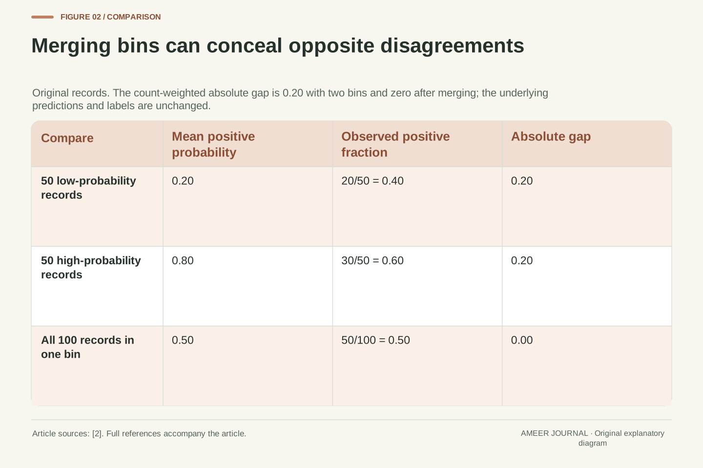
Construct a new set of one hundred records. Fifty receive a positive probability of 0.2, but twenty of those fifty are positive: their observed fraction is 0.4. The other fifty receive 0.8, but thirty of them are positive: their observed fraction is 0.6. Each group differs from its assigned probability by twenty percentage points, in opposite directions.

Now put all one hundred predictions into one bin. The average probability is (50 × 0.2 + 50 × 0.8) ÷ 100 = 0.5. The positive fraction is also (20 + 30) ÷ 100 = 0.5. The single plotted point sits exactly on the diagonal, concealing the two disagreements that were visible when the groups stayed separate.

For an explicit summary, define the gap as the count-weighted average of each bin's absolute difference. The two-bin result is 0.5 × 0.2 + 0.5 × 0.2 = 0.2; the one-bin result is zero. The predictions did not improve. Only the grouping changed. The curve documentation makes bin count and strategy explicit choices. [2] Keep those choices with a reported chart or gap, and inspect more than one coarse summary before treating a diagonal point as strong evidence.

Let B₁ contain fifty predictions p=0.2 with twenty positive labels, and B₂ contain fifty predictions p=0.8 with thirty positives. Their reliability points are (0.2,0.4) and (0.8,0.6). Each absolute gap is 0.2. Define our diagnostic G=Σ_b(n_b/N)|p̄_b−f_b|. With these two bins, G=0.5·0.2+0.5·0.2=0.2.

Merge the bins without changing any underlying record. The merged mean probability is 0.5, the merged positive fraction is 0.5, and G becomes zero. This is exact cancellation before the absolute value is taken. It is a counterexample to interpreting a small coarse-bin gap as proof of agreement at every represented probability. Our retained table also makes the grouping reproducible rather than treating a chart as an independent observation.

The documented curve routine exposes n_bins and a uniform/quantile strategy [2]; our G is an explicitly defined local calculation, not a claim about that routine returning a particular scalar. Choosing finer groups can reveal disagreement but also leaves fewer records per group. Preserve bin membership or enough information to reconstruct it, and report counts alongside the points. This example establishes dependence on the grouping rule without claiming that any one bin count is universally optimal.

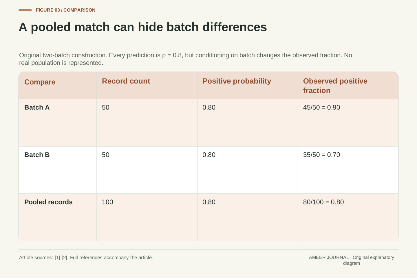
Grouping only by predicted probability can also hide differences between kinds of records. Return to predictions of 0.8 for everyone. This time, define two batches of fifty. Batch A contains forty-five positives, a fraction of 0.9. Batch B contains thirty-five positives, a fraction of 0.7. Together they contain eighty positives out of one hundred, so the overall probability and positive fraction both remain 0.8.

The single overall point is unchanged, but neither batch matches it. The prediction understates the positive frequency in A by ten percentage points and overstates it in B by ten percentage points. This is an original counterexample showing why agreement after one kind of grouping does not establish agreement after every other useful grouping.

The batch labels here are invented. In a real evaluation, a meaningful grouping could follow a documented capture condition or a defined use case, provided the records and outcomes support that question. Keep the group definition, count and result together. A small group may be noisy, and repeatedly searching many groupings can produce striking patterns by chance. The example calls for a clear question and further evidence; it does not identify a real system's failure or declare that every possible subgroup must be inspected identically.

Construct two labelled groups, A and B, each with n=50 and constant assigned positive probability p=0.8. Let their positive counts be 45 and 35. The conditional empirical fractions are f_A=0.9 and f_B=0.7, while the pooled fraction is (45+35)/100=0.8. Thus conditioning only on the common predicted probability produces exact empirical agreement, but conditioning additionally on the group exposes gaps of magnitude 0.1.

The group-weighted absolute gap is 0.1, whereas the pooled gap is zero. Both results refer to the same prediction/label table and are compatible. The counterexample shows that the conditioning information forms part of the question. It does not require assuming that these arbitrary groups represent demographic categories, capture devices or any measured deployment population.

For an actual investigation, specify why a group definition is relevant and retain counts and selection rules. Interpret apparent differences with attention to sample size and the number of comparisons considered; this article supplies no significance test or multiple-comparison procedure. A probability-only reliability curve is useful for its stated conditional summary, but it cannot prove every stronger conditional property. Keep that boundary explicit rather than treating an aggregate point as a certificate that all parts of the evaluated population behave alike.

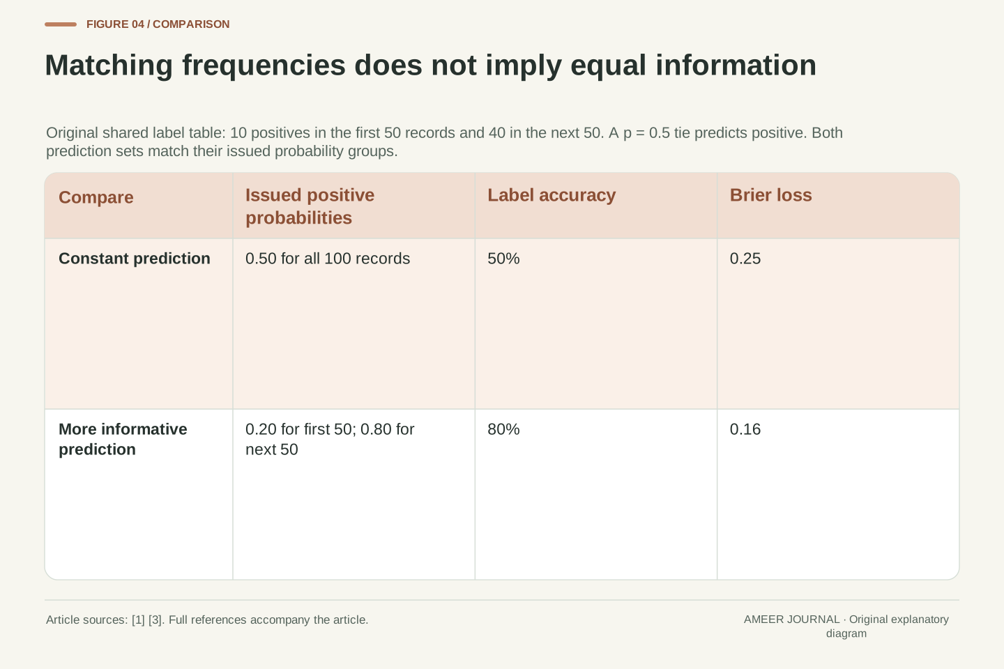
Consider another hundred-record table with fifty positives overall. Its first fifty records contain ten positives; its second fifty contain forty. A prediction set that assigns 0.5 to everyone matches the overall positive fraction exactly. A second set assigns 0.2 to the first group and 0.8 to the second. Those two probability groups also match their respective observed fractions exactly.

Both sets therefore agree with the frequencies at the probability values they issue in this constructed sample. The second set is more informative about differences between records. Under our stated rule that a 0.5 tie predicts positive, the constant set gets fifty labels right. The varying set predicts negative for the first group and positive for the second, getting forty right in each group: eighty in total.

Their Brier scores differ too: 0.25 for the constant set and 0.16 for the varying set. This is the promised example of why a probability score and a calibration diagnosis are not interchangeable. The official guide makes that broader distinction between reliability and discriminatory information. [1] Here the full table shows the mechanism directly. A useful evaluation asks both whether the stated probabilities agree with outcomes and whether the predictions distinguish cases in a way relevant to the task.

Use the same balanced label table for two prediction structures: fifty records contain ten positives and fifty contain forty. Predictor C assigns p=0.5 to all records. Predictor D assigns 0.2 to the first group and 0.8 to the second. C's sole probability group has f=0.5; D's two probability groups have f=0.2 and f=0.8. Both display exact empirical reliability at their issued probabilities.

Their informational resolution differs. With the declared positive-on-tie threshold, C has accuracy 0.5 and BS=0.25. D correctly labels forty negatives in the first group and forty positives in the second, giving accuracy 0.8. Its squared probability loss is 0.16 in each group and overall. The lower score does not arise from correcting a probability-group discrepancy in C; D separates cases that C gives the same probability.

This construction illustrates the official guide's caution that Brier loss combines aspects beyond calibration [1]. It also connects to the preceding subgroup example: probability-only agreement is a weaker property than agreement conditional on additional information. None of these finite tables proves a population property. They demonstrate why a comparison should retain the prediction structure, outcome labels and metric definitions, rather than treating one scalar loss or a diagonal point as a complete assessment of usefulness.

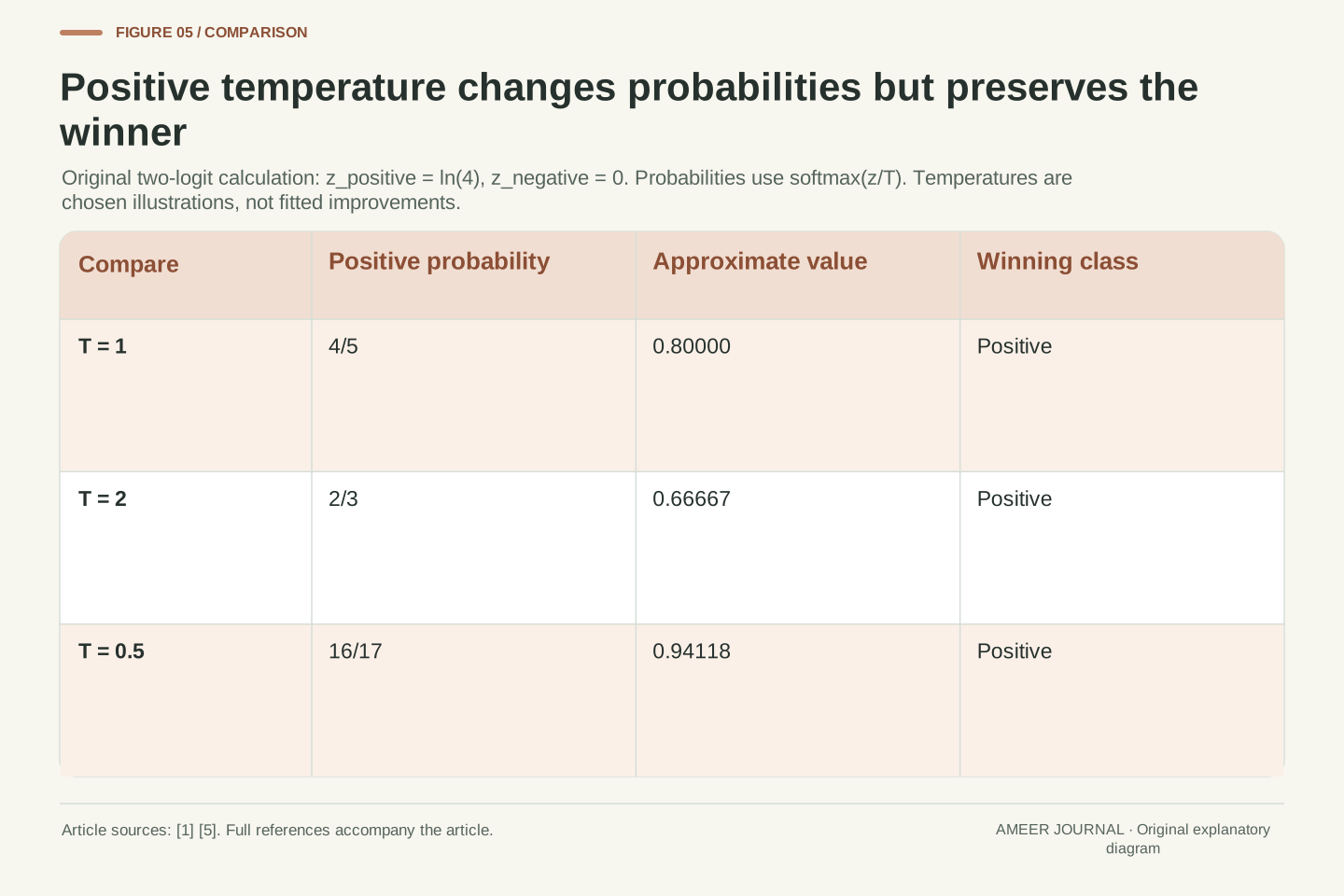
Temperature scaling changes the conversion from a model's numerical class scores, called logits, into probabilities. The documented form divides the logits by a positive temperature before applying softmax. [1] To see the effect without training anything, use two invented logits: ln(4) for “bicycle present” and zero for “absent”. At temperature one, the positive probability is 4 ÷ (4 + 1) = 0.8.

At temperature two, the corresponding ratio becomes 2 ÷ (2 + 1), about 0.66667. At temperature one half, it becomes 16 ÷ (16 + 1), about 0.94118. The positive class wins all three times. A common positive scaling preserves which logit is largest, while the probabilities change. That explains how a calibration procedure can alter probability quality without changing the selected class.

Our three temperatures are chosen examples, not fitted improvements. In the documented calibration procedure, the temperature is learned using a separate calibration set. [1] The 2017 paper by Guo and colleagues reported useful temperature-scaling results on the datasets it studied. [5] That historical finding does not make every chosen temperature beneficial or guarantee that a present-day model will be calibrated on a different population.

For logits z and a common T>0, temperature scaling uses softmax(z/T). The actual mathematical block is retained from the official guide [1]. Division by a positive scalar preserves the ordering within the logit vector, and exponentiation is strictly increasing, so the maximizing class remains unchanged. This statement concerns class ordering within a prediction, not a universal claim about every calibration method or cross-sample metric.

Choose z_positive=ln4 and z_negative=0. At T=1, p_positive=4/5. At T=2, exp(ln4/2)=2, so p_positive=2/3. At T=1/2, exp(2ln4)=16, so p_positive=16/17. All three probabilities exceed 1/2, preserving the positive label under the declared decision rule. Our local calculation reproduces these exact ratios; it does not execute a model or estimate an optimal T.

The guide describes fitting temperature by minimizing log loss on held-out calibration data [1]. Guo et al.'s 2017 paper record reports temperature scaling's effectiveness on its studied classification datasets [5], not a timeless guarantee across models and distributions. Distinguish the algebraic property of unchanged argmax from the empirical question of improved probability estimation. The former follows from T>0; the latter requires a specified fitting procedure and evaluation on appropriate independent data.

The opening table was designed to make the arithmetic transparent. Once we know it contains eighty positives, assigning 0.8 everywhere matches that table's overall frequency. Reporting this match as proof that we discovered a reliable predictor would confuse using the answers with demonstrating a result on new cases. The example establishes a calculation, not a prediction achievement.

In an actual calibration workflow, the classifier has training data, the probability adjustment has fitting data, and the final assessment needs evidence appropriate to the intended use. The official guide explains why calibration fitting should use predictions from data independent of the classifier's training data, and describes held-out or cross-validation approaches. [1] A final check should also remain separate from choices tuned using its own answers. Repeatedly changing the adjustment after inspecting the test results turns those results into development information.

Keep the model version, adjustment method, fitted parameters, record selection and evaluation date together. If the kinds of incoming images change, an old reliability plot remains evidence about its original records. It does not automatically describe the new ones. This is why a calibration result should name its population and conditions instead of becoming a permanent confidence label attached to the model's name.

Fitting and evaluation have different evidential roles. In the opening construction, selecting a constant p equal to the known empirical positive fraction minimizes that table's constant-prediction Brier loss. The optimization follows algebraically from the recorded labels. Evaluating that same choice on the same labels does not establish out-of-sample calibration or demonstrate that a learned representation identifies bicycles.

The official guide separates classifier training from calibrator fitting and explains why using the classifier's training predictions can bias the adjustment [1]. Held-out predictions or an appropriately designed cross-validation procedure address that fitting boundary. A final evaluation must also reflect the model-selection process: outcomes used repeatedly to choose methods, parameters or reporting groups have participated in development. Our recommendation is to retain those roles explicitly rather than labelling every reused record “test data”.

Record the classifier identity, calibrator, parameters, data partitions and target population. Distinguish the population described by an evaluation from any later population on which predictions will be used. An observed relationship between p and y is conditional on how those records were produced and selected; changing that context requires fresh evidence. This article performs no fitting or sampling experiment. Its constructions isolate measurement effects so that an actual evaluation can report its own data and validation design without inheriting claims from the examples.

Begin with the event: what does the positive label mean, and which probability belongs to it? Then inspect the outcomes, record count and decision rule. Accuracy tells you about the resulting labels. A reliability diagram compares average probabilities with observed positive fractions. Brier and log loss retain probability information using different formulas. Their definitions and conventions belong beside the values. [2][3][4]

Our examples show why the rest of the record matters. Two sets can share 80 percent accuracy but score 0.16 and 0.1961 under the binary Brier formula. Merging two bins can reduce a declared gap from 0.2 to zero without changing a prediction. Two batches can disagree in opposite directions while their pooled fraction matches. A constant 0.5 prediction can agree with an overall frequency while failing to distinguish records as well as more informative predictions do.

Finally, ask how any adjustment was fitted and where it was checked. Keep the original probabilities, labels and group assignments so another person can reproduce the report. A meaningful uncertainty assessment connects each conclusion to its actual calculation and data. It leaves room to say that a label was correct, a probability was overconfident on a sample, or an overall average missed a subgroup difference without treating those observations as the same result.

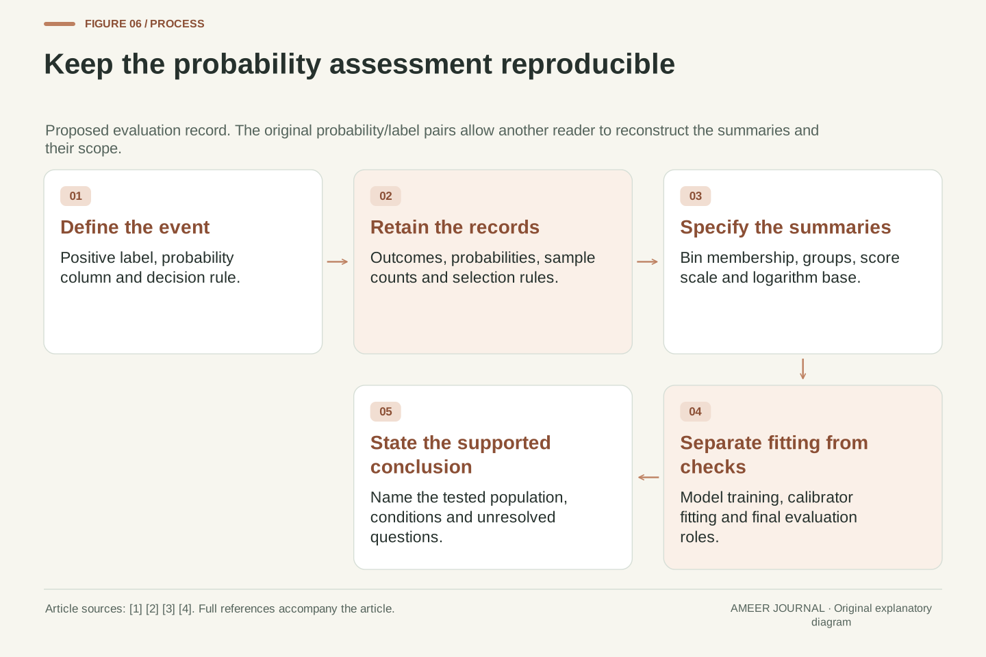
A reproducible probability assessment specifies the positive event, probability column, target labels, decision rule, record selection and sample count. Add the reliability-bin definition, group conditioning, binary or multiclass scoring convention and logarithm base. The cited APIs make these distinctions concrete: calibration curves use positive-label fractions, Brier scaling depends on the declared convention, and log loss uses a stated probability and logarithm definition [2][3][4].

The retained original examples yield equal classification accuracy 0.8 with Brier losses 0.16 and 0.1961; a two-bin absolute-gap average of 0.2 versus a merged gap of zero; subgroup fractions 0.9 and 0.7 hidden within a pooled 0.8; and two empirically probability-group-matched predictors with losses 0.25 and 0.16. The positive-temperature calculation changes probabilities from 4/5 to 2/3 or 16/17 while preserving the winning class. These outcomes answer different measurement questions.

Retain the fitting/evaluation boundary and the conditions under which each result was obtained. A probability report is stronger when it can be reconstructed from the original prediction/label pairs and interpreted at the correct level of conditioning. The goal is a scoped judgment about the evidence available: which labels were correct, how probabilities related to outcomes, which groups were examined and what the evaluation leaves unresolved.