What you’ll take away
- Known-noise inversion and generation from a noisy state are different information problems.
- The forward mixture uses cumulative schedule coefficients; unweighted subtraction gives the wrong result.
- Noise, clean-sample and v targets need their matching reconstruction formulas.
- A predicted clean sample is distinct from the next stochastic state sent through the loop.
- Representation, conditioning, schedule and decoding settings are part of an interpretable diffusion result.
The model makes a prediction; the scheduler decides the next state
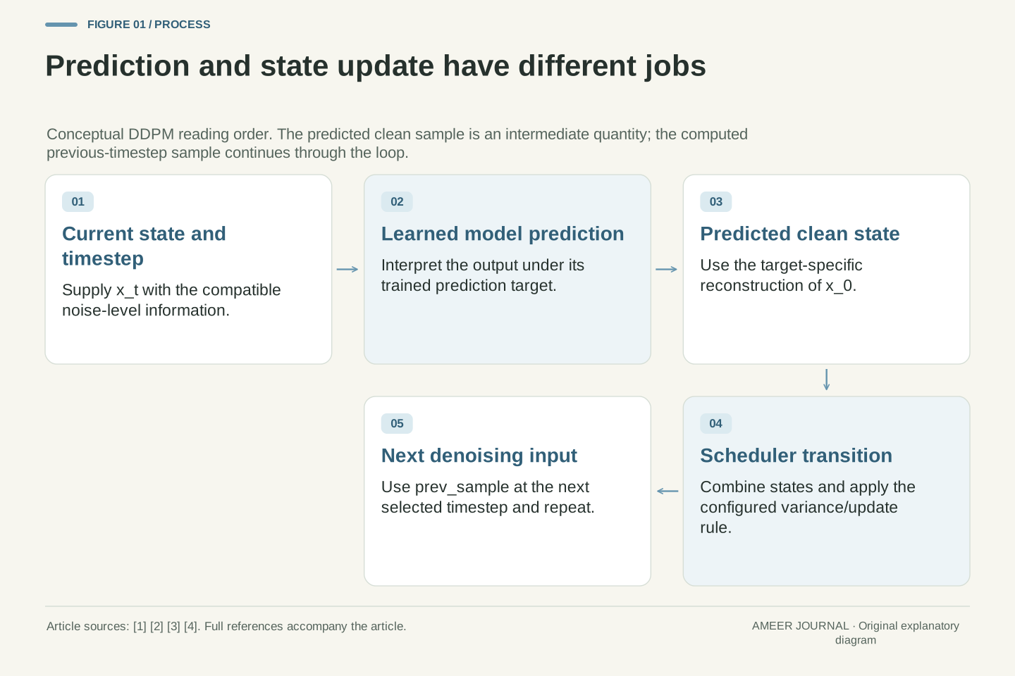
A diffusion image generator is often described as starting with noise and gradually removing it. That sketch leaves two jobs inside one sentence. In the documented DDPM pipeline, a learned model predicts a noise-related quantity from the current state and its timestep. A scheduler uses that prediction, the current state and the configured update rule to calculate the next state. The result returns to the model for another prediction. [2][4]
The distinction becomes clearer with a tiny original calculation. We use only two numerical coordinates, not a photograph. A clean pair of (0.25, −0.25) and a noise pair of (1, −1) combine, under stated weights, into (0.8, −0.8). If we know the exact added noise, we can recover the clean pair algebraically. During generation, that clean pair and its exact forward noise are not supplied as the answers to the model.
This article explains the DDPM mechanism using pinned Diffusers version 0.35.1 documentation and source code. The original DDPM authors describe models trained to gradually denoise data. [1] Our coordinate examples expose the arithmetic behind that idea; they are not a model run, generated photograph or claim that every modern image-generation method uses the same sampler.
Separate the learned denoiser from the numerical update. In the documented DDPM inference loop, the model consumes a sample and timestep and produces an output interpreted by the configured prediction target. The scheduler combines that output with the current state and its schedule to compute a previous-timestep state; that state becomes the next model input [2][4]. A prediction of x₀ and an actual next sampler state are distinct objects.
Our original construction uses x₀=(1/4,−1/4), ε=(1,−1) and a cumulative signal coefficient parameter ᾱ=16/25. The forward mixture produces x_t=(4/5,−4/5). Exact recovery is straightforward when ε is supplied. The generative problem differs because the denoiser must infer an appropriate output from its inputs rather than being handed this constructed clean/noise decomposition.
We use the pinned Diffusers 0.35.1 DDPM implementation as a concrete reference, alongside the original authors' description of parameterized chains trained to denoise [1][3]. All reported numerical results come from local rational or floating-point arithmetic on stipulated coordinates. No network was trained, no pretrained checkpoint was loaded and no scheduler library was executed. This scope allows precise comparisons without generalizing one DDPM parameterization to every diffusion, flow or distilled image-generation system.
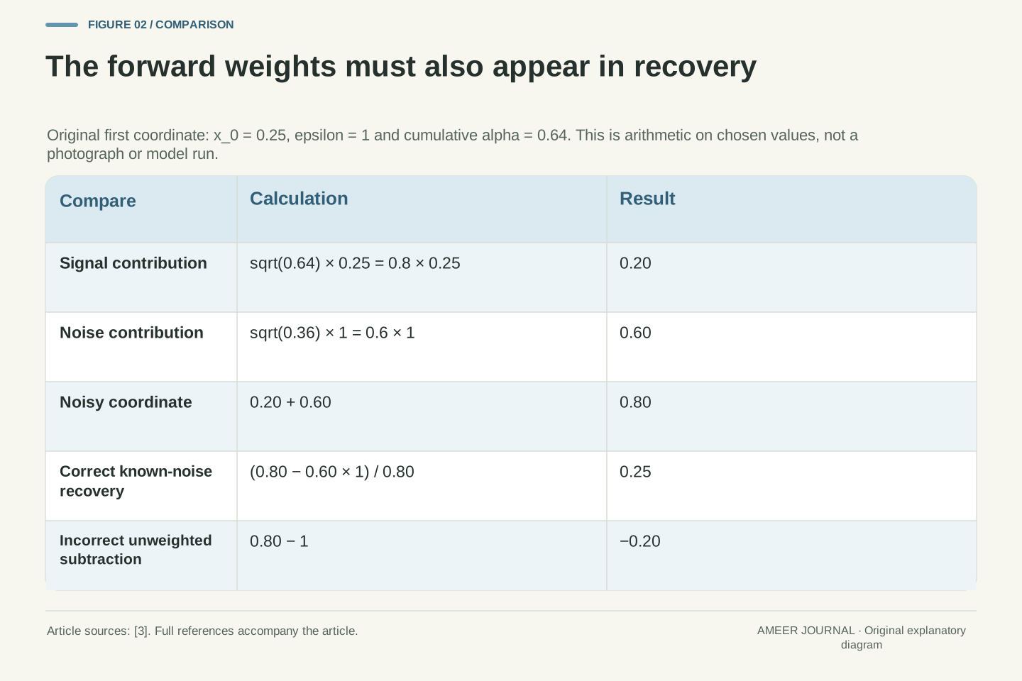
The forward mixture uses two weights, not an unweighted addition
For our chosen noise level, multiply each clean coordinate by 0.8 and each noise coordinate by 0.6, then add the results. The first coordinate becomes 0.8 × 0.25 + 0.6 × 1 = 0.8. The second becomes −0.8. These weights follow the DDPM forward-noising formula: the square root of the cumulative alpha multiplies the clean data, and the square root of one minus that value multiplies the noise. [3]
Because the cumulative alpha is 0.64, the weights are √0.64 = 0.8 and √0.36 = 0.6. Their squares add to one, while the weights themselves add to 1.4. This is not a recipe saying that 64 percent of pixels remain untouched or that two percentages must sum to one. Both terms can affect every coordinate in the numerical array.
If we know the noise exactly, recovery must undo both operations. Subtract 0.6 × 1 from the first noisy coordinate, then divide by 0.8: (0.8 − 0.6) ÷ 0.8 = 0.25. Simply subtracting the unweighted noise gives 0.8 − 1 = −0.2, which is the wrong result. The schedule's coefficients are part of the calculation, not optional decoration.
The implementation's add_noise method computes x_t=√ᾱ_t x₀+√(1−ᾱ_t)ε using the cumulative alpha at the requested timestep [3]. With ᾱ_t=16/25, define s=4/5 and n=3/5. Our exact two-coordinate mixture is s(1/4,−1/4)+n(1,−1)=(4/5,−4/5). The coefficients satisfy s²+n²=1; they do not constitute a convex combination with s+n=1.
Given the stipulated ε, the algebraic inverse for s>0 is x₀=(x_t−nε)/s. It recovers (1/4,−1/4). Unweighted subtraction x_t−ε instead gives (−1/5,1/5), demonstrating why “remove the noise” is underspecified unless the noise target and scale are known. These are coordinate operations, not statements that a particular fraction of image locations is left unchanged.
The same formula can produce noisy values outside a normalized clean-data range. It is not automatically a display-ready pixel blend. The cited training example normalizes its clean images into [−1,1] before noising [5]; other representations require their own conventions. Our coordinates and noise values are explicitly selected for arithmetic clarity, not sampled to estimate a Gaussian distribution or used as a visual model-quality experiment.
A timestep's cumulative alpha is not just its last step's alpha
The word “cumulative” matters. The pinned scheduler forms alpha values from one minus each beta and multiplies the alphas across the schedule. [3] To make the distinction visible, choose three illustrative alpha values: 0.9, 0.9 and 64/81, which is about 0.790123. Their successive products are 0.9, 0.81 and 0.64.
At the third position, the cumulative value is therefore 0.64 even though the last individual alpha is about 0.790123. The clean coefficient used in our forward mixture is the square root of 0.64, or 0.8. Using the last individual alpha in its place would describe a different calculation. These three values are a small constructed schedule, not recommended settings for an image model.
The timestep tells the denoiser and scheduler where the current state belongs in that schedule. It is not a percentage of the image that has become correct. The documented pipeline sets an inference timestep sequence and passes its entries through the denoising loop. [2][4] A useful record keeps the actual sequence and schedule together. Merely writing “step three” leaves out which coefficients and state that step represents.
The pinned constructor defines α_t=1−β_t and computes ᾱ_t as the cumulative product of the alphas [3]. Choose the original three-entry schedule α=(9/10,9/10,64/81). Its cumulative products are (9/10,81/100,16/25). At the final entry, the step alpha is 64/81 while the cumulative alpha is 16/25. Substituting one for the other changes both signal and noise coefficients.
This schedule also supplies the preceding cumulative value 81/100 for our later reverse-transition calculation. The associated final step beta is 17/81. All values are stipulated to make the algebra exact; they are not defaults, tuned parameters or a proposal for replacing a trained model's schedule. The source implementation and documentation distinguish training timestep count, inference timestep selection and the current state passed to step [2][3].
The label t therefore has meaning through the compatible model and scheduler configuration. Counting loop iterations alone does not identify ᾱ_t, the previous selected timestep or the model-output interpretation. Preserve the schedule and timestep sequence when comparing results. Our construction demonstrates the cumulative-product relationship without running a training process or assuming that a shorter inference sequence can be produced by deleting arbitrary updates from every model family.
One noisy pair can come from more than one clean-and-noise pair
Our first coordinate was 0.8 because 0.8 × 0.25 + 0.6 × 1 = 0.8. But another combination gives the same result: 0.8 × (−0.5) + 0.6 × 2 = 0.8. Apply the matching signs to the second coordinate and both constructions produce the same noisy pair, (0.8, −0.8), from different clean pairs and different noise pairs.
This is an original arithmetic counterexample to the idea that the noisy array alone carries an obvious, uniquely labelled noise layer waiting to be removed. If someone supplies the exact noise used in either construction, its corresponding clean pair can be recovered. If that information is missing, the equation alone does not choose between the constructions.
A learned denoiser brings information acquired during training to the prediction problem. The DDPM authors describe learning the parameters of the generative denoising process. [1] Our two constructions do not show that a particular trained model would consider both possibilities equally likely. They show the narrower reason learning matters: successful algebra with a known noise target is a different problem from predicting an appropriate target from a noisy state, timestep and any supported conditioning information.
The map from a pair (x₀,ε) to x_t is not one-to-one when both components are unknown. At the same coefficients s=4/5 and n=3/5, our original pair x₀=(1/4,−1/4), ε=(1,−1) gives x_t=(4/5,−4/5). The alternative x₀′=(−1/2,1/2), ε′=(2,−2) gives exactly the same x_t. Both computations are retained as exact rational arithmetic.
This demonstrates underdetermination of the decomposition, not equal posterior probability under a particular data distribution. A learned model can assign different plausibility to candidate clean states using its training-derived structure and conditioning. The original DDPM description explicitly places learning in the generative denoising process [1]. The equation by itself does not supply that learned information.
The distinction also explains why knowledge of a numerical starting state is not automatically knowledge of a desired clean image and its forward corruption. Exact inversion of a supplied training pair uses information unavailable in the ordinary generation question. Our construction does not rule out specialized reconstruction or inversion procedures; it isolates the missing-information issue in the elementary formula. Nor does it establish a claim about memorization, originality or ownership of actual model outputs, which would require evidence beyond these two coordinates.
Training knows the added noise because the training code created it
The documented training example starts with clean training images, generates noise, chooses a timestep and uses the scheduler to create a noisy input. The model predicts the noise from that input and timestep. Its prediction is compared with the noise that the training code actually added, using a mean squared error loss. The optimizer then updates the model's parameters. [5]
There is no mystery about where the target comes from in that exercise. The training code retained it when making the noisy example. That does not mean the denoiser receives the correct answer as an input. In the cited loop, the noisy images and timesteps go into the model, while the known noise is used separately to calculate the loss. [5] The difference between the prediction and this target supplies a learning signal.
Generation uses the learned model in a different role. The documented inference loop begins with random noise and repeatedly alternates prediction with a scheduler update. [4] It does not begin by selecting a hidden clean photograph and handing its exact added noise to every denoising call. Our tiny example makes the distinction concrete: we can calculate an exact target because we invented the clean/noise pair; an actual denoiser must produce its output from the inputs its generation pipeline supplies.
In the pinned training guide, clean_images come from the prepared dataset, noise is sampled with the same tensor shape, and a timestep is sampled for each image. add_noise constructs the input at that noise level. The network is called with the noisy images and timesteps, and its output is compared with the retained noise using mean squared error before backpropagation and an optimizer step [5]. These are separate input, target, loss and parameter-update roles.
This explicit construction makes noise prediction a supervised target within the example. The training code knows ε because it sampled ε; the model is not directly supplied ε as its answer. Matching our exact mixture's known target illustrates the loss relationship but is not an experiment in whether a neural network can learn it. We did not perform any optimization or evaluate a checkpoint.
The inference guide instead initializes a noisy state and loops through a selected sequence, passing each model output to the scheduler [4]. Model evaluation within that loop does not itself constitute the training procedure above. Keep a training noise schedule, sampled training timesteps, optimizer iterations and inference update count distinct. Their names all refer to progress through some process, but they do not count the same operation or establish the same computational workload.
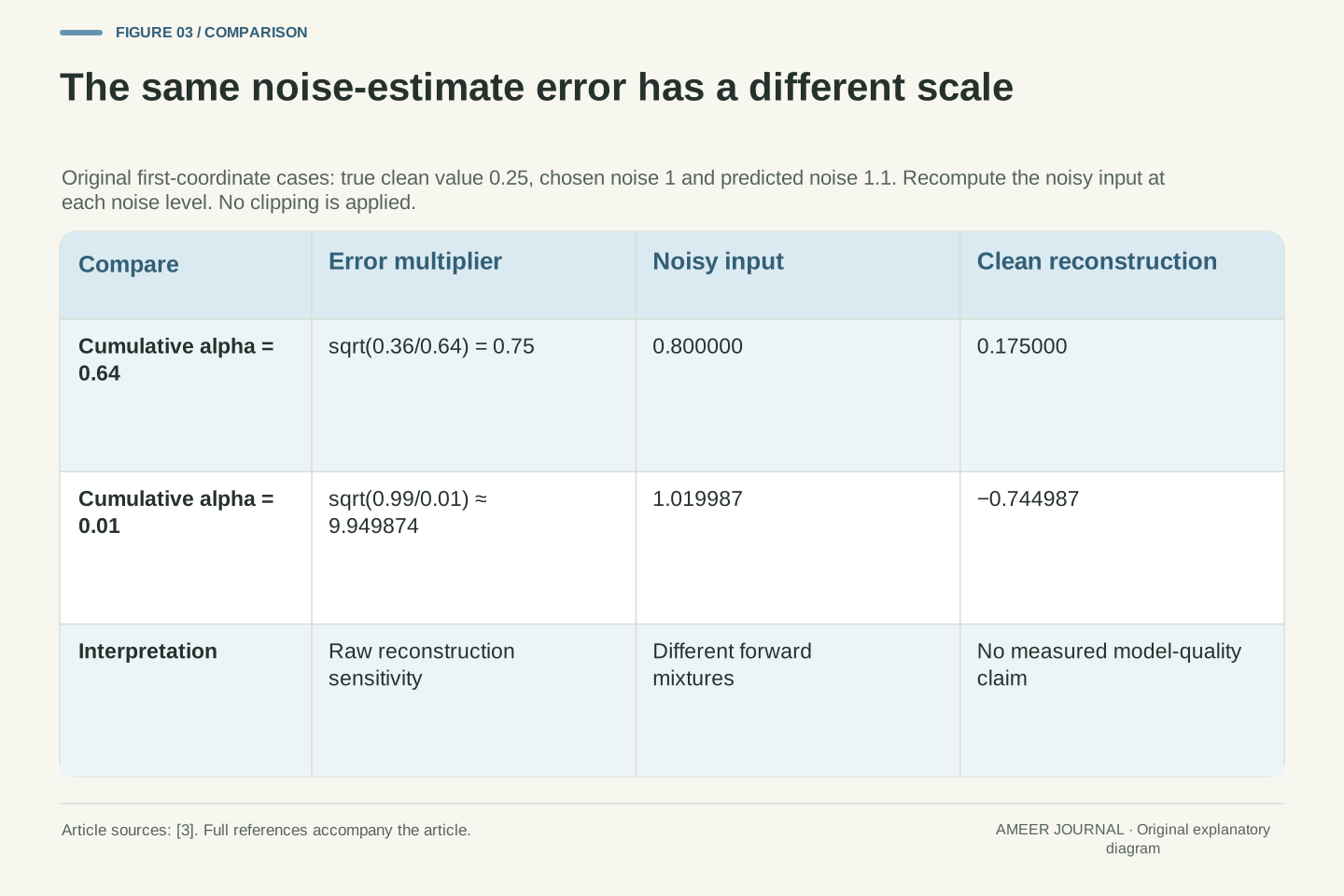
An error in the noise estimate changes the clean estimate by a scale-dependent amount
Return to the first coordinate, whose true clean value is 0.25 and chosen noise is 1. Suppose the predicted noise is 1.1, an error of 0.1. With our 0.8 and 0.6 coefficients, the reconstructed value becomes (0.8 − 0.6 × 1.1) ÷ 0.8 = 0.175. Its error is −0.075. The same noise-prediction error does not translate into the same-sized clean-value error.
Now construct another noise level with cumulative alpha 0.01. Its clean coefficient is 0.1 and its noise coefficient is √0.99, about 0.99499. Using the same clean value, chosen noise and prediction error produces a clean estimate of about −0.74499, nearly one unit below 0.25. The new noisy coordinate was calculated for this new noise level; we did not reuse the old 0.8 input.
These results follow from the inverse formula implemented for the noise-prediction branch. [3] They illustrate its sensitivity at the stated noise levels before any clipping or thresholding. They do not show that a real model makes equal errors at every timestep, or that visual image quality follows directly from one coordinate's error. Those would be additional empirical claims.
For 0<ᾱ_t<1, let the predicted noise be ε̂=ε+δ. Substitution into x̂₀=(x_t−√(1−ᾱ_t)ε̂)/√ᾱ_t gives x̂₀−x₀=−√((1−ᾱ_t)/ᾱ_t)δ. This is an exact algebraic consequence of the documented epsilon branch [3], before clipping or thresholding. It identifies a sensitivity multiplier, not a model-error distribution.
At ᾱ=0.64, the multiplier is 0.6/0.8=0.75. With δ=(0.1,−0.1), the clean error is (−0.075,0.075), and reconstruction is (0.175,−0.175). At ᾱ=0.01, the multiplier is √99≈9.949874. The separately recomputed noisy pair is approximately (1.019987,−1.019987), and the same δ yields reconstruction (−0.744987,0.744987).
The code also has clipping and thresholding branches, which our calculation does not apply [3]. The examples therefore isolate the raw algebra rather than reporting every effect of a configured scheduler. They neither assert equal denoiser error across timesteps nor convert coordinate error into a perceptual-quality score. A real comparison would need the actual model outputs, representation, noise levels and update settings. Retaining those boundaries prevents a useful sensitivity calculation from becoming an unsupported performance claim.
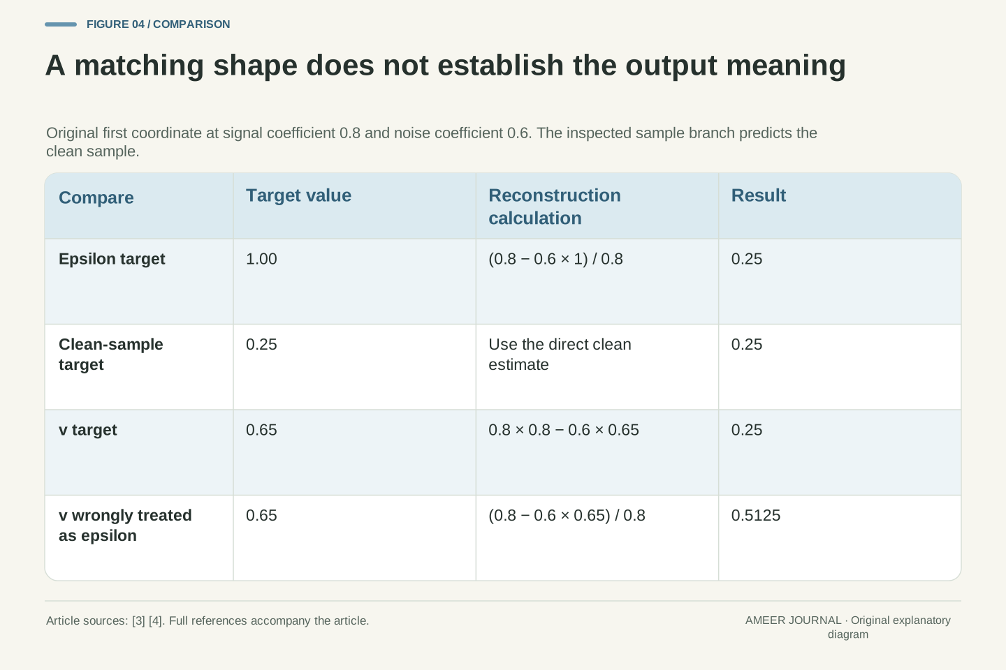
Noise, clean sample and v are different meanings for a model output
A numerical output is useful only when the scheduler knows what it represents. The inspected DDPM source has branches for noise prediction, direct clean-sample prediction and a third combination called v-prediction. [3] They are different ways to express information about the same noisy state. A vector with the correct shape can still be interpreted incorrectly if the configured target does not match how the model was trained.
For the first coordinate of our example, the noise target is 1 and the clean target is 0.25. The v target is 0.8 × 1 − 0.6 × 0.25 = 0.65. Using the documented v formula, the clean value is recovered as 0.8 × 0.8 − 0.6 × 0.65 = 0.25. The three target numbers differ, even though they describe the same constructed state.
If we mistakenly treat 0.65 as a noise prediction, the noise-based formula produces (0.8 − 0.6 × 0.65) ÷ 0.8 = 0.5125. The calculation runs, but it answers the wrong question. The lesson is to match the model-output meaning to the scheduler configuration. The direct-sample meaning used here follows the actual inspected implementation branch; a loose description of “the sample” is not enough to establish which state it names.
The pinned step implementation distinguishes prediction_type='epsilon', 'sample' and 'v_prediction' [3]. Its operative sample branch assigns model_output directly to pred_original_sample; we therefore interpret that branch as a prediction of x₀, rather than adopting the inconsistent “noisy sample” wording in a parameter description. The epsilon branch uses (x_t−nε̂)/s, and the v branch uses sx_t−nv̂.
With v=sε−nx₀, our exact example has ε=(1,−1), x₀=(1/4,−1/4) and v=(13/20,−13/20). The v reconstruction yields x₀ because s²+n²=1. Misinterpreting v as epsilon instead yields (41/80,−41/80), or (0.5125,−0.5125). This is an original controlled target-mismatch example, not an observed configuration error in a released model.
Prediction semantics are determined by the compatible model and scheduler, not merely by tensor dimensions or an output attribute's name. The pipeline guide accesses a model result through .sample while using it as a noise residual [4], illustrating why that attribute alone is insufficient. Record the prediction target explicitly and apply its corresponding transformation. No claim is made that the DDPM v parameterization is the definition of every “velocity” target used by other generative model families.
A predicted clean sample is not the next sample in the loop
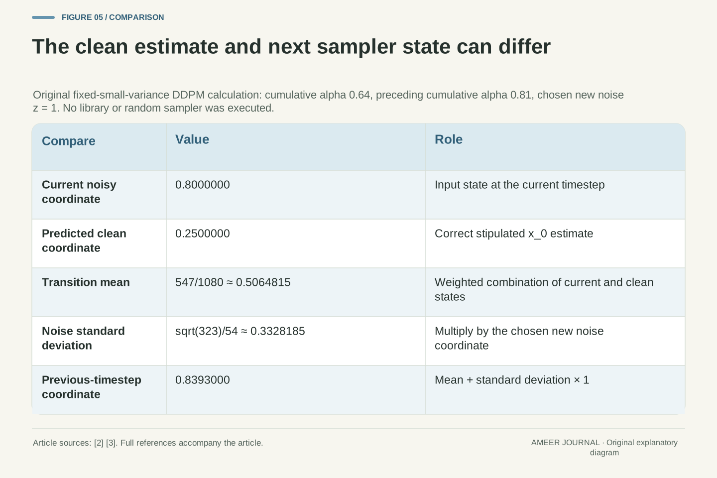
Suppose the model predicts our clean value perfectly as 0.25. A DDPM update still has another calculation to perform. The source combines the clean estimate with the current noisy state using schedule-dependent coefficients, and a stochastic transition can add newly generated noise. The API exposes the predicted clean sample and the previous-timestep sample separately; the latter is the state passed into the next loop iteration. [2][3]
Use our current cumulative alpha of 0.64 and preceding value of 0.81. For the first coordinate, the constructed transition's mean is about 0.50648. Its noise standard deviation is about 0.33282. If we stipulate a new noise coordinate of 1, the next sample is about 0.83930. That is neither the predicted clean value of 0.25 nor the incoming noisy value of 0.8.
These are calculations from the documented fixed-small-variance formulas with chosen inputs, not a library run or a randomly sampled experiment. They show why a preview of predicted clean content and the actual next numerical state must not be confused. A particular stochastic update also need not move every coordinate closer to our chosen clean reference. Its role belongs to the configured sampling process, not a promise of visibly improving every individual number at every step.
Take ᾱ_t=16/25 and ᾱ_prev=81/100. The effective step alpha is 64/81 and beta is 17/81. From the pinned DDPM coefficients, the predicted-clean multiplier is 85/162 and the current-sample multiplier is 38/81 [3]. For x̂₀=1/4 and x_t=4/5, the conditional mean is (85/162)(1/4)+(38/81)(4/5)=547/1080≈0.5064815.
For the stipulated fixed-small-variance transition, variance is (1−ᾱ_prev)/(1−ᾱ_t) times the effective beta, giving 323/2916. Its standard deviation is √323/54≈0.3328185. Choosing the new noise coordinate z=1 gives a previous sample of approximately 0.8393000. The mirrored second coordinate uses z=−1. These values are algebraically reconstructed from the source formulas; no scheduler object or stochastic draw was executed.
The source's variance-addition line is retained in the exact native code as well as the surrounding extracted evidence. pred_original_sample and prev_sample remain separate outputs [2][3]. Our clean estimate lies inside the ordinary clip range, and the arithmetic does not apply extra thresholding. Do not replace the next-state result with x̂₀ merely because x̂₀ looks closer to a desired final image. The following denoiser call expects the state associated with the selected timestep and update scheme.
The numbers being denoised may be latent coordinates rather than visible pixels
Our two coordinates are mathematical values, not a miniature photograph. Real pipelines also need a clear interpretation of their arrays. The basic DDPM example in the guide works with an image-sized array. Its Stable Diffusion example instead denoises a smaller latent representation and uses a separate decoder to turn the result into an image. [4] A latent coordinate should not automatically be read as a particular displayed pixel.
The documented latent example divides image height and width by eight. For a requested 512-by-512 image, that gives a 64-by-64 spatial grid. There are 4,096 locations in that grid, compared with 262,144 in the final image: a factor of 64 in spatial location count. This is an arithmetic description of that example, not a claim that all models use the same factor or that computation becomes exactly 64 times faster.
Channel counts, precision and model operations also affect storage and work. The decoder is another operation with its own learned behavior. The guide additionally applies scaling around its latent decoding step. [4] When inspecting a noisy tensor, a predicted clean tensor or a preview, establish which representation you are looking at. A display conversion can make numbers visible without making that display the state expected by the next denoising call.
The pipeline guide contrasts a basic DDPM sample in image space with a Stable Diffusion example that denoises latent representations before VAE decoding [4]. Representation is therefore part of the meaning of x_t and x̂₀. The algebra of a noise parameterization does not establish that their coordinates are already display pixels, nor does an arbitrary visualization preserve the pipeline's input convention.
In the documented example, each requested image dimension is divided by eight when the initial latent tensor is created. For 512×512 output, the spatial grid is 64×64: 4,096 versus 262,144 spatial positions. The position-count ratio is 64, not eight. This calculation deliberately excludes channels, dtype and model compute; it is not a memory-footprint or inference-speed ratio. Other encoders or pipelines may use different compression and scaling conventions.
The source includes an explicit latent scaling step before decoding and a separate conversion to a displayable image [4]. Keep these transformations distinct from the scheduler's own state update. Our original two-coordinate calculations specify their representation abstractly, so they cannot predict image texture, compression artifacts or decoder behavior. A model comparison must preserve the actual tensor conventions and decoding path rather than treating visually similar previews as proof that two intermediate states have the same numerical meaning.
A prompt conditions a prediction; it does not become the missing noise answer
Text-to-image generation adds another input to the prediction process. In the guide's Stable Diffusion example, a tokenizer and text encoder produce embeddings from the prompt. Those embeddings condition the denoising model, helping steer its output towards the requested content. [4] The prompt is not an exact list of the random values that were added to some already chosen clean photograph.
The example also uses conditional and unconditional predictions for classifier-free guidance. It combines those predictions before passing the result to the scheduler. [4] That places guidance in a specific part of the process: it modifies the prediction used for the numerical update. It does not eliminate the need for a compatible prediction target, current timestep, schedule and decoder.
This distinction helps when comparing settings in an image generator. A different prompt, guidance setting, sampler or inference sequence can change a different part of the calculation. A progress preview alone does not identify which part changed. Keep the model and the relevant settings attached to the result you are assessing. Our arithmetic demonstrates how a chosen prediction affects a state; it does not measure prompt adherence, image realism or whether increasing any particular setting improves an actual generator.
In the guide's text-conditioned example, tokenization and a text encoder produce embeddings supplied to the conditional denoiser [4]. This extends the model's inputs without supplying the unknown clean/noise decomposition as ground truth. Conditioning can influence the predicted residual, but it does not change which numerical target the scheduler expects that residual to represent.
The documented classifier-free-guidance loop obtains conditional and unconditional predictions and combines them before scheduler.step [4]. The distinction between prediction construction and state propagation remains intact. The guided output, current sample and timestep feed the update, and the resulting state continues through the chosen inference sequence before decoding. This describes the cited example rather than declaring that every image generator uses an identical guidance formulation or architecture.
When diagnosing a changed result, identify which component or setting changed: model weights, condition encoding, guidance, prediction parameterization, scheduler, timestep sequence or representation/decoder. A comparison that changes several of these simultaneously cannot attribute its result to one of them from the final image alone. Our calculations do not provide an optimal guidance scale, preferred sampler or perceptual benchmark. They establish enough separation between the components to formulate such an empirical comparison precisely and retain the settings needed to interpret it.
Ask which state an intermediate result is supposed to represent
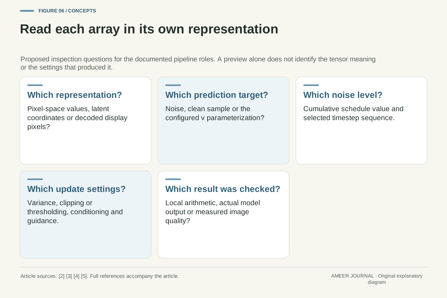
The most useful question when inspecting a diffusion run is often, “What does this array represent here?” It could be a current noisy state, a noise prediction, a direct clean estimate, a v prediction, a next sampler state or decoded pixels. Several can have compatible-looking dimensions while requiring different formulas. The inspected scheduler and pipeline expose those distinctions in their operations and outputs. [2][3][4]
Our worked example shows the consequences. The noisy first coordinate is 0.8, its chosen noise is 1, its clean value is 0.25 and its v value is 0.65. Interpreting v as noise produces the wrong 0.5125 reconstruction. Even a correct clean estimate of 0.25 can lead to a next stochastic state of about 0.83930 under the stated transition and chosen new noise. None of those values is contradictory once its role is named.
Keep the model identity, representation, prediction target, schedule and timestep sequence with a result. Record any clipping, guidance and decoding settings relevant to the comparison. Then distinguish exact arithmetic checks from evidence about generated image quality. DDPM denoising becomes easier to reason about when “remove noise” is unpacked into a learned prediction and a precisely defined update, each operating on the right state.
An interpretable trace names the state at each boundary: model input x_t, model output under its configured target, reconstructed x̂₀, previous selected-timestep sample and decoded output. The source distinguishes these roles through add_noise, the target-dependent reconstruction branches, update coefficients, variance addition and the two scheduler outputs [3]. The inference guide shows how those outputs participate in the loop [4].
The original exact values provide a compact consistency check: x₀₁=1/4, ε₁=1, x_t₁=4/5 and v₁=13/20. Correct target interpretation recovers 1/4; using v as epsilon yields 41/80. The stipulated reverse transition has mean 547/1080 and variance 323/2916, producing approximately 0.8393000 at the selected new-noise coordinate. These are local formula results, not a proof that a learned model predicts the correct target on real images.
A reproducible comparison retains compatible model/configuration identities, representation scaling, target semantics, timestep sequence, stochastic inputs and relevant clipping, guidance and decoding choices. It also identifies what was actually executed and which outcomes were measured. Our construction supplies arithmetic evidence about those interfaces while leaving model quality and perceptual success to appropriate experiments. That separation lets a reader investigate a diffusion result without mistaking a known-target inversion for the complete generative task.
Sources & further reading
Explore the references behind this guide. External pages may change after our review.
- Denoising Diffusion Probabilistic ModelsJonathan Ho, Ajay Jain and Pieter Abbeel · Accessed 7 Nov 2026
- DDPMScheduler · Hugging FaceHugging Face Diffusers developers · Accessed 7 Nov 2026
- DDPM scheduler source — Diffusers v0.35.1Hugging Face Diffusers developers · Accessed 7 Nov 2026
- Understanding pipelines, models and schedulers · Hugging FaceHugging Face Diffusers developers · Accessed 7 Nov 2026
- Train a diffusion model — Diffusers v0.35.1Hugging Face Diffusers developers · Accessed 7 Nov 2026
Article updated 7 Nov 2026.
Found something we should revisit?
Good explanations get better with thoughtful feedback.