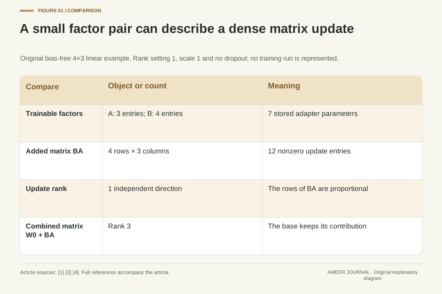
A LoRA adapter can contain far fewer trainable numbers than the weight matrix it adjusts. That does not mean it chooses a few entries in that matrix and leaves all the others untouched. Its two factors combine to form an update. In the small example below, seven factor entries produce an update that changes all twelve entries of a four-by-three weight matrix. The update has rank one, while the combined weight matrix still has rank three. Those statements describe different properties and can all be true at once.

The original LoRA method keeps the base weight matrix frozen while training smaller factors whose product supplies an added update. [1] We will use a bias-free linear layer and explicit numbers to follow that product through one input. Dropout is absent and the initial scale is one. This is an analytical example, not a model-training result. Its purpose is to make three practical distinctions visible: how many factor entries are trainable, how many entries of the effective matrix change, and which base weights are still needed to use the adapter. Once those objects are kept separate, parameter counts, adapter files and merged models become much easier to compare without assigning them the same meaning.

LoRA parameterizes an update to a frozen base matrix rather than selecting a sparse subset of its entries. For W0 of shape d×k, factors A of shape r×k and B of shape d×r produce an update sBA, where s is the declared scaling coefficient [1][2]. The rank bound applies to that update. It does not generally constrain the rank of W0+sBA to r, and it does not imply that only r or r(d+k) entries of the effective weight matrix change.

We analyze a bias-free 4×3 linear map with r=1, s=1 and no dropout. Seven stored factor parameters produce twelve nonzero update entries. Exact arithmetic then shows rank(BA)=1 but rank(W0+BA)=3. No optimizer, training dataset or model inference is involved. The same construction supports a forward-pass comparison, a merge identity and a wrong-base example. We also separate factor parameter counts from the storage of base weights and from total runtime memory. This distinction matters when interpreting a small adapter checkpoint: a compact representation of a change is not, by itself, a standalone replacement for the model to which that change belongs.

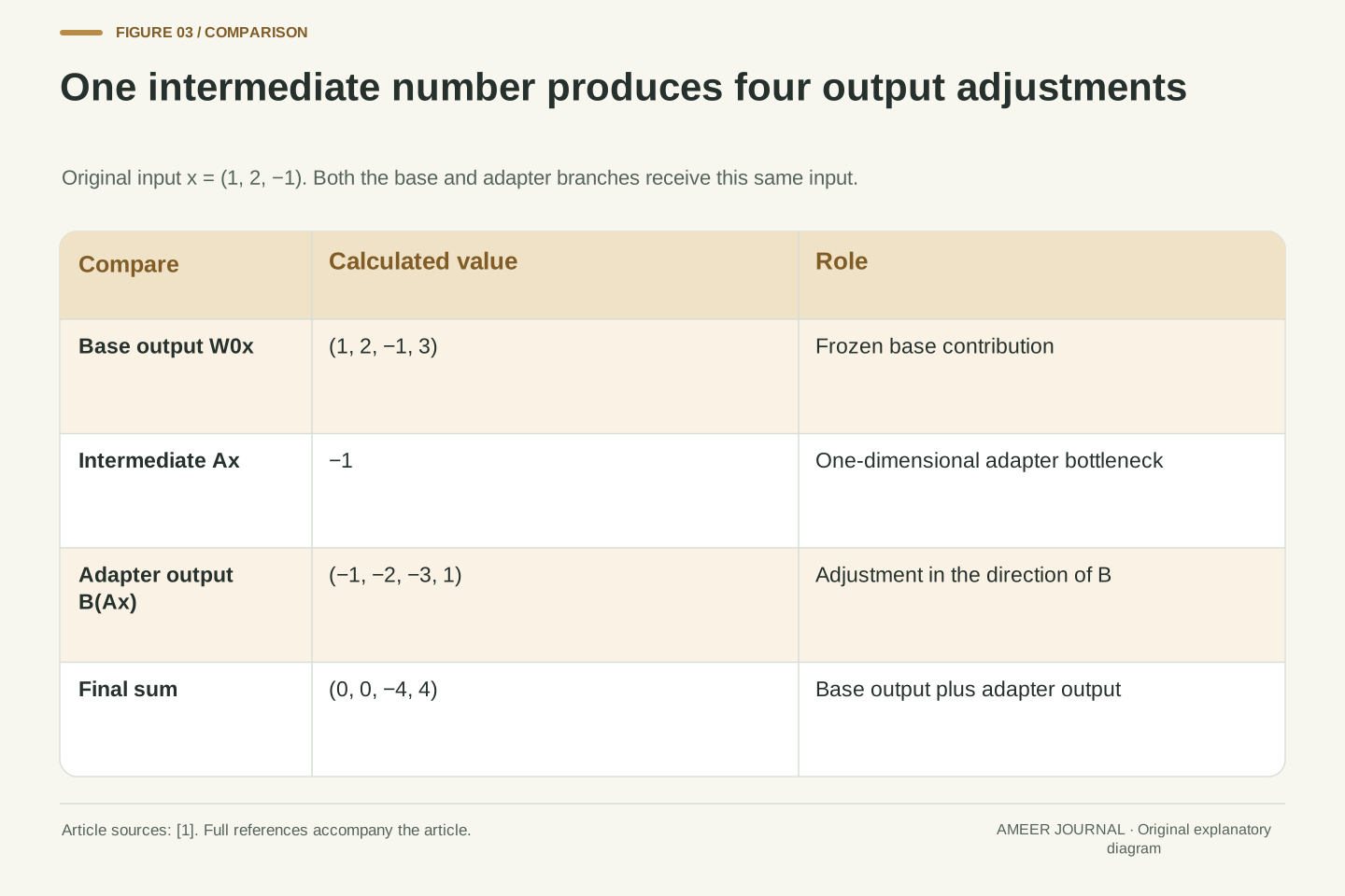
Our input has three numbers: x=(1,2,−1). The base matrix W0 has four rows: (1,0,0), (0,1,0), (0,0,1), and (1,1,0). Each row takes a weighted sum of the input. The first row returns 1, the second 2, the third −1, and the fourth 1+2=3. Therefore the base output is (1,2,−1,3). Four output coordinates come from three input coordinates; that is why the matrix is four by three.

Now define the adapter factors. A is the single row (2,−1,1). B is the single column (1,2,3,−1). A first reduces the three-number input to one number, and B expands that number to four output adjustments. The size of this intermediate space is our chosen rank setting, one. We will add those adjustments to the base output, rather than feeding the base output through the adapter. That parallel use of the same input is part of the LoRA construction. [1] Keeping the matrix shapes visible prevents a common mental mix-up: the adapter's small intermediate dimension does not change the layer's final output size. It still returns four numbers, ready for the same downstream interface.

Use column-vector convention with x=[1,2,−1]^T and W0 rows [1,0,0], [0,1,0], [0,0,1], [1,1,0]. Thus W0∈R^(4×3) and W0x=[1,2,−1,3]^T. The bias term is omitted deliberately, so every change in this example is attributable to the matrix update. We do not rely on a framework's stored-weight orientation; the stated mathematical convention defines the multiplication.

Let A=[2,−1,1]∈R^(1×3) and B=[1,2,3,−1]^T∈R^(4×1). Then Ax has dimension one and B(Ax) has dimension four. The adapted linear map is y=W0x+B(Ax) at scale s=1. Both branches receive x; the adapter is not applied to W0x [1]. The factor bottleneck therefore changes the parameterization of the update without changing the map's 3-input/4-output contract. A real implementation must additionally match its weight-storage convention. The referenced PEFT configuration, for example, distinguishes layers storing weights with input/output dimensions reversed [2]. That API detail should be resolved when mapping this column-vector algebra to tensors, rather than silently transposing one factor and trusting shapes that happen to multiply.

First multiply A by the input. The calculation is 2×1+(−1)×2+1×(−1)=−1. The adapter's intermediate result is one number, −1. Multiply it by B to obtain (−1,−2,−3,1). These are adjustments to the four base-output coordinates. Adding them to (1,2,−1,3) gives the final result (0,0,−4,4).

Notice what rank one allows here. All four output adjustments can be nonzero, but they must follow the same fixed direction B for this fixed adapter. Another input changes the scalar produced by A. It scales that direction instead of independently choosing four unrelated adjustments. For example, the input z=(1,2,0) gives Az=0, so its adapter adjustment is the zero vector even though the factors themselves are nonzero. This is a constraint on how the update responds across inputs, not a rule that one output coordinate changes. A low-rank update can therefore be broad in where it acts while restricted in the kinds of changes it can express. The two views become consistent once we follow the multiplication rather than interpreting “one” as a count of edited weights.

The intermediate scalar is Ax=2(1)−1(2)+1(−1)=−1. Hence BAx=B(−1)=[−1,−2,−3,1]^T and y=[1,2,−1,3]^T+[−1,−2,−3,1]^T=[0,0,−4,4]^T. Every operation follows the stated shapes and fixed scale. The calculation directly verifies the adapter branch without forming the full update matrix first.

For arbitrary input v, BA v lies in the span of B. Since A and B are nonzero here, the update's image is one-dimensional. That dimensional constraint coexists with nonzero values in all four output coordinates. Inputs in the null space of A receive no update; z=[1,2,0]^T is one example because Az=2−2=0. Thus the adapter can change every effective matrix entry while leaving some particular inputs' outputs unchanged. This observation is about a linear map, not a quality prediction for an adapted language model. It explains the structural capacity being restricted: the factorization ties the response directions together. Counting affected coordinates or inspecting one changed output vector would not recover that rank constraint, because rank describes the map over its full input space.

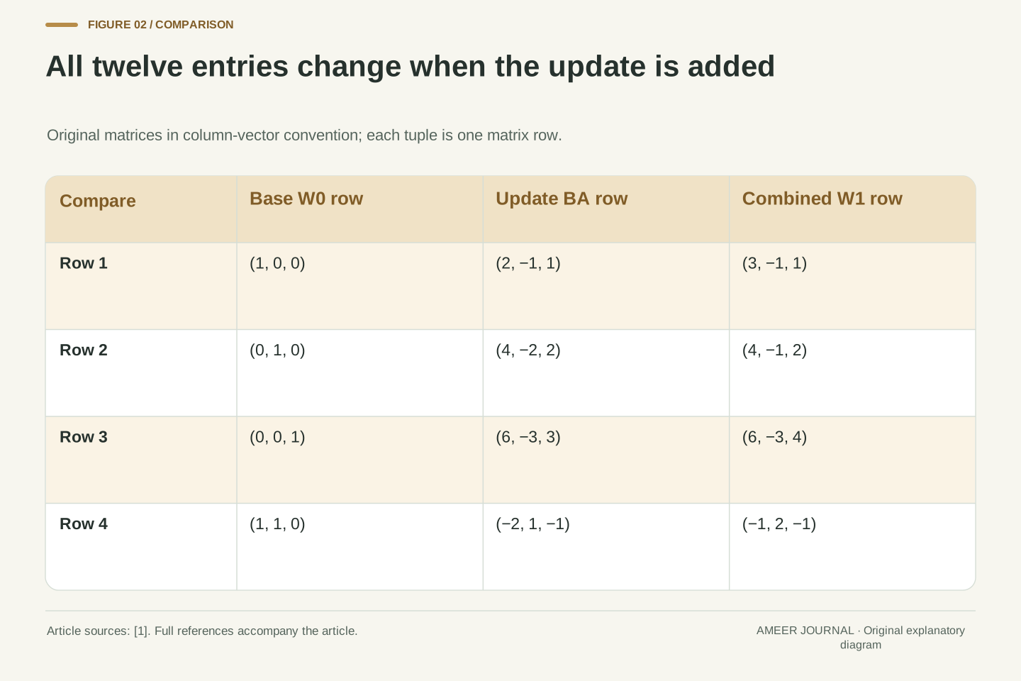
Form the full update by multiplying the column B by the row A. Its rows are (2,−1,1), (4,−2,2), (6,−3,3), and (−2,1,−1). All twelve entries are nonzero. Yet every row is a multiple of the first row, so the update has rank one. It can be dense and low rank at the same time. Dense means its entries are nonzero in this example; low rank describes the dependence between its rows or columns.

Adding this update to W0 gives rows (3,−1,1), (4,−1,2), (6,−3,4), and (−1,2,−1). These rows are no longer all multiples of one row. The first three form a three-by-three matrix with determinant 4, which is nonzero, so the combined matrix has rank three. Three is its maximum possible rank because it has only three columns. You do not need to calculate determinants to use an adapter, but this check makes the distinction exact. LoRA restricts the form of the added change in this setup. It has not compressed the entire original transformation into a one-dimensional map. The base matrix continues to contribute its own structure after the update is added.

The outer product BA has rows [2,−1,1], [4,−2,2], [6,−3,3], [−2,1,−1]. Each of its 12 entries is nonzero, and every row is a scalar multiple of A. Because neither factor is zero, rank(BA)=1. This is an explicit counterexample to equating a low-rank parameterization with a sparse effective update.

The merged matrix W1=W0+BA has rows [3,−1,1], [4,−1,2], [6,−3,4], [−1,2,−1]. Its top 3×3 minor has determinant 4. Therefore rank(W1)≥3; with only three columns, rank(W1)=3. The base matrix also has rank 3 because its first three rows form the identity. The update rank and the combined rank are consequently different objects even in a single small layer. Factor parameters are not unique either: replacing A with 2A and B with B/2 preserves BA exactly. This scaling freedom shows why a count of stored factor entries is not the same as a count of uniquely identifiable degrees of freedom in the resulting matrix. For checkpoint accounting we still count all stored entries; for rank and expressiveness we inspect the product they represent.

Our four-by-three base matrix contains twelve entries. A rank-one A contains three and B contains four, so the adapter contains seven trainable factor entries. Those seven values describe the twelve-entry update through multiplication. If the base stays frozen, twelve base entries still exist, but they are not the entries being adjusted by the adapter optimizer. Microsoft’s reference workflow explicitly marks LoRA parameters as trainable and saves those parameters separately. [4]

The general count for a d-by-k matrix and rank setting r is r×k+d×r, or r(d+k). A full matrix has d×k entries. This does not guarantee a saving for every chosen shape and rank. In our tiny example, rank two would require 2×3+4×2=14 factor entries, more than the twelve entries of the full matrix. For a larger illustrative case, a 4096-by-4096 matrix has 16,777,216 entries. Rank eight requires 8×4096+4096×8=65,536 factor entries: one 256th of the base count, or 0.390625%. That is a count for one specified matrix, not for an entire model. To produce a whole-model count, identify every adapted layer and include any other parameters that the configuration also trains.

For the declared 4×3 map, a full trainable weight matrix has dk=12 entries, whereas the r=1 factorization stores rk+dr=3+4=7 trainable entries. The base W0 remains stored and frozen. These counts describe parameter tensors, not a count of nonzero entries in the effective update: all twelve entries of BA are nonzero in the worked construction. Microsoft’s reference instructions separately mark adapter parameters as trainable and save an adapter-only state [4].

The factor-entry inequality for a strict saving is r(d+k)<dk. For d=4,k=3, this requires r<12/7, so r=1 saves entries while r=2 stores 14 and does not. In a separate 4096×4096, r=8 example, dk=16,777,216 and r(d+k)=65,536. The ratio is 1/256=0.00390625, or 0.390625%. This is a per-matrix parameter comparison under the stated target and rank. PEFT exposes target-module selection, additional trainable modules and bias settings [2]; each affects what belongs in a whole-model accounting. Summing only one factor pair while labeling the result as total trainable model size would change the scope of the measurement. Conversely, counting the frozen base as if every one of its entries were an adapter optimizer variable would erase the distinction the parameterization is designed to make.

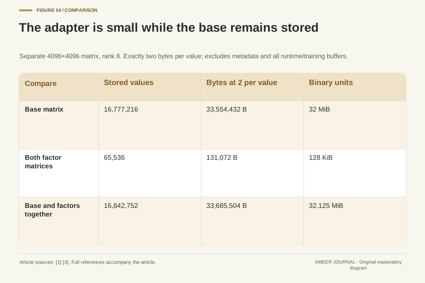
Keep the larger example and assume every stored value occupies exactly two bytes. The 4096-by-4096 base then needs 33,554,432 bytes, or 32 MiB. The rank-eight factors need 131,072 bytes, or 128 KiB. Storing both takes 32.125 MiB for these weight values. The adapter is small beside the base, but using the two together has not reduced this matrix’s stored values to 128 KiB. The original transformation remains part of the computation.

That distinction explains an adapter download that looks surprisingly tiny. PEFT’s checkpoint documentation says its adapter state does not contain the base model, and loading the adapted model requires the original model as well. [3] Our byte arithmetic excludes file headers, configuration, activations, gradients, optimizer state and runtime buffers. Those exclusions matter when estimating memory needed to train or serve a complete model. A count of trainable factor values cannot by itself predict peak device memory. It does, however, answer a precise storage question: how many numerical values must be kept for this particular change? If several compatible adapters share one retained base, their separate change files may be much smaller than several complete adapted checkpoints. The shared base and the configuration needed to connect each change to it still belong in the deployment record.

Assume two bytes per stored numerical value for the separate 4096×4096, r=8 example, with identical precision for base and factors. Base storage is 16,777,216×2=33,554,432 bytes=32 MiB. Factor storage is 65,536×2=131,072 bytes=128 KiB. Their sum is 33,685,504 bytes=32.125 MiB. These exact binary-unit conversions concern the specified weight values only. They are not a measured checkpoint size or VRAM result.

PEFT’s adapter checkpoint state excludes the base weights, while the base remains necessary to instantiate the adapted model [3]. An adapter-only file therefore describes an increment relative to a dependency, not a self-contained compressed substitute. Training and inference memory have additional components, including activations and implementation-specific buffers; training may also retain gradient and optimizer-related tensors. Parameter freezing and a reduced optimizer population should not be translated into a fixed total-memory reduction without measuring the actual workload. Likewise, files can carry metadata or use different stored precisions, so the two-byte assumption must remain attached to the example. For a collection of adapters, separate the shared base cost from each adapter's marginal storage. That accounting makes the benefit interpretable without claiming that the original layer or its data representation has disappeared.

The worked example used scale one. Keep A, B and x fixed, but multiply the adapter contribution by two. The base output remains (1,2,−1,3), while the adjustment becomes (−2,−4,−6,2). The new total is (−1,−2,−7,5). The update still has rank one; changing this nonzero scale changes its magnitude, not the number of independent directions it can express. This is a useful distinction when two adapters have the same rank setting but produce different adjustments.

For ordinary LoRA scaling, the referenced PEFT configuration uses alpha divided by r. It also offers a rank-stabilized option using alpha divided by the square root of r. [2] Record the actual convention instead of inferring scale from the rank alone. Initialization is another separate choice. The documented default sets B to zero, making the initial added update zero before training. [2] Our nonzero factors were chosen for arithmetic, not obtained from that initialization by a training run. A rank setting of one is an upper bound on the product’s rank; if one factor is zero, the product has rank zero. Therefore the configuration’s rank value, the current product’s actual rank and the update’s scale are related but distinct pieces of information.

Write the fixed linear map as y=W0x+sBAx. For our factors, replacing s=1 with s=2 changes the output from [0,0,−4,4]^T to [−1,−2,−7,5]^T. Multiplication by a nonzero scalar preserves the rank of BA; s=0 instead gives a zero update. Scale therefore controls a different aspect of the map from the bottleneck dimension r.

PEFT v0.17.0 documents ordinary scaling alpha/r and the use_rslora alternative alpha/sqrt(r) [2]. This article uses the declared scalar directly, so it does not compare training outcomes under those conventions or recommend an alpha value. The same reference documents default zero initialization of B, yielding a no-op adapter before training. Even with configured r=1, B=0 gives rank(BA)=0. More generally, rank(BA)≤r, with equality depending on the factors. Our hand-selected nonzero factors realize equality and are not claimed as learned weights. Preserve rank, scaling policy and initialization as separate configuration fields. A larger configured r changes shapes and the available update family, but does not itself establish larger effective updates, better task quality or a particular training trajectory.

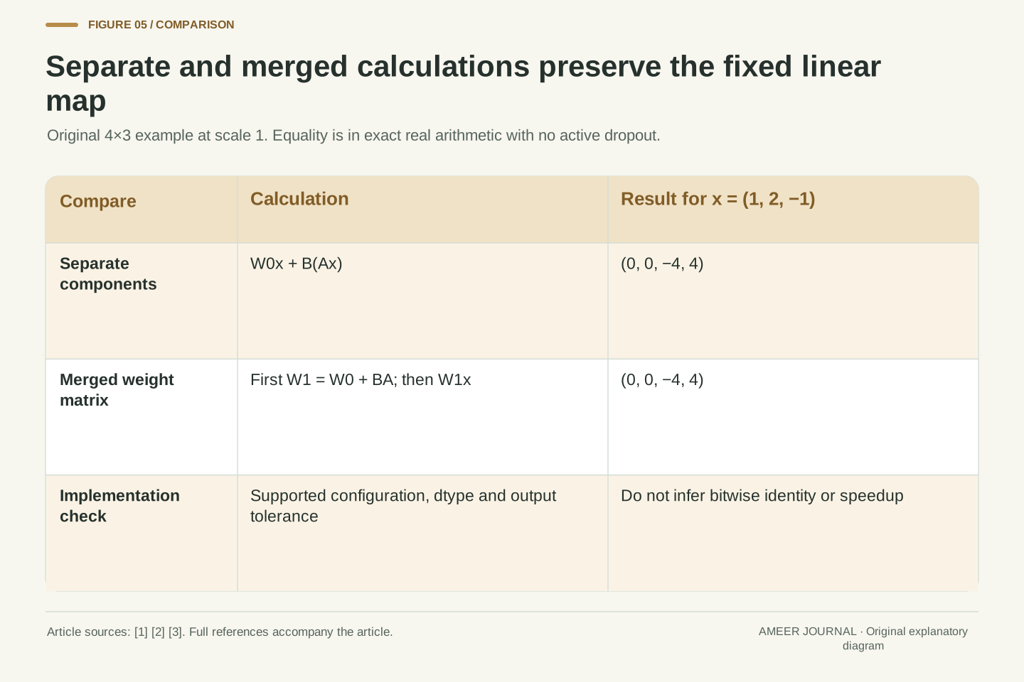
For our fixed layer, there are two equivalent ways to calculate the output. One keeps W0, A and B separate, calculates the base and adapter branches, and adds their results. The other first creates W1=W0+BA, then multiplies W1 by the input. The rows of W1 were listed earlier. Applying them to (1,2,−1) gives (0,0,−4,4), exactly the same result as the separate branches. The equality holds for every input in this real-number linear construction, not only for the example we chose.

This is the algebra behind merging a LoRA update into base weights. The original paper discusses that operation, and PEFT documents a merge_and_unload method. [1][2] A merged weight matrix has the original matrix shape; it is not an adapter-only checkpoint. Our calculation assumes a fixed scale and no active dropout. Real implementations also have numerical precision, supported layer types and configuration restrictions. PEFT warns that some settings, including certain quantization techniques, do not support merging. [3] Therefore use the actual method’s contract and compare outputs in the intended configuration. The algebra explains what merging should preserve; it does not promise identical floating-point bits or a particular speedup on every system.

Distributivity gives W0x+sBAx=(W0+sBA)x for fixed linear factors and scalar s. At s=1, the explicitly formed W1 yields [0,0,−4,4]^T on our example input, agreeing with the separately evaluated branches. This identity holds for arbitrary x in exact real arithmetic. It is not restricted to the one test vector, and it does not require the combined matrix to inherit the adapter’s low rank.

The fixed-update interpretation underlies the paper’s merge construction and PEFT’s merge_and_unload interface [1][2]. Our scope excludes active stochastic dropout or other input-dependent changes to the adapter branch. Finite-precision evaluation may also round the separate and merged operation sequences differently, so algebraic equality is not a claim of bitwise identity for every implementation. The PEFT checkpoint guide additionally states that some method/configuration combinations cannot merge, including certain quantization settings [3]. A deployment should verify support and compare representative outputs at its actual dtype and tolerance. The resulting weight matrix has shape 4×3 in our example and contains the base contribution as well as the update. It therefore represents a full adapted layer, while the stored A/B factors alone remain a relative change requiring their base.

Suppose someone keeps our same adapter but changes the first entry of W0 from 1 to 2. The base matrix still has four rows and three columns, so all the multiplications still fit. For x=(1,2,−1), however, the final output becomes (1,0,−4,4) instead of (0,0,−4,4). The adapter file did not change. The difference came from the base to which it was applied. Matching shapes alone cannot establish that the intended combined transformation has been reconstructed.

PEFT’s checkpoint format separates adapter weights from adapter configuration and includes information about the base model. Microsoft’s reference instructions likewise load the pretrained checkpoint and then the LoRA checkpoint. [3][4] Preserve the actual base version, factor weights, target layers and scaling configuration together. A model name without the relevant revision may be less precise than the experiment record needs. If you merge and unload, retain the original components separately when you need them for later comparisons or switching. The PEFT documentation explains that the returned merged model no longer has its adapter-specific methods, such as disabling or unmerging an adapter. [3] A small change file and a full merged model serve different storage and workflow purposes, even when they represent the same intended adaptation.

Let W0′ equal W0 except that its first-row, first-column entry increases from 1 to 2. Both bases have identical shapes, but applying the unchanged factors to the same x gives (W0′+BA)x=[1,0,−4,4]^T. The earlier result was [0,0,−4,4]^T. The difference is exactly [x1,0,0,0]^T for arbitrary input. This constructed case demonstrates that structural compatibility of tensor dimensions does not establish base-weight identity or behavioral equivalence.

The adapter checkpoint must therefore be interpreted with its base dependency and configuration. PEFT documents adapter weights and configuration separately, including base-model information; Microsoft’s reference loading sequence restores the pretrained state before the adapter state [3][4]. Preserve the precise base revision and target-module mapping alongside rank, scale and any additionally trained parameters. For an exported merged model, record that the artifact now contains the adapted full weights. PEFT’s merge_and_unload result loses PEFT-specific functionality, including the ability to disable or unmerge the adapter through those methods [3]. Retaining separate original components is a proposed reproducibility practice, not a claim that the exported object remembers them. This distinction avoids treating a successfully loaded shape-compatible adapter as proof that the intended model state has been recovered.

The arithmetic has established several useful facts about one declared layer. Seven trainable factor entries can create twelve nonzero update entries. The added matrix has rank one, while the combined matrix has rank three. Separate and merged calculations produce the same linear function under the stated assumptions. The larger storage example shows why a small adapter can be convenient to keep while its base remains necessary. None of those calculations tells us which rank will produce the best answers on a real task.

For that decision, record what was adapted, what was trained and how the result was evaluated. Keep the dataset and target definitions clear, compare useful task behavior, and measure memory or speed with the actual workload if those are selection criteria. The LoRA reference implementation notes that the best configuration can depend on architecture and task. [4] A larger factor count provides a different update family, but quality also depends on the data and training process. Our worked example gives a precise vocabulary for discussing the choice: update rank, combined matrix, trainable entries, base dependency and merge state. Use those labels in experiment records so a smaller file or a larger rank setting does not silently become a claim about model quality.

The exact construction establishes parameter, rank and algebraic identities, not an empirical rank-selection rule. For the specified nonzero factors, rank(BA)=1; rank(W0+BA)=3; the factor count is 7 and the dense update contains 12 nonzero entries. For the separate 4096-square case, rank 8 yields 65,536 factor entries while retaining 16,777,216 base entries. These quantities can guide an experiment’s accounting, but they do not determine task accuracy, convergence, latency or peak memory.

An evaluation record should specify the base revision, adapted matrices, per-layer ranks and scales, initialization, any extra trainable biases/modules, training objective and data, and the task-level evaluation protocol. Microsoft’s implementation guidance explicitly leaves configuration choices dependent on architecture and task [4]. Compare candidate settings under a controlled protocol, and measure resource outcomes rather than substituting parameter ratios for them. Distinguish the factor checkpoint from the merged artifact used during measurement; a different representation can change the implementation path while preserving the intended real-valued linear map. The practical contribution of the example is this separation of objects. It makes a claim about a compact update inspectable, and leaves claims about a useful adapted model to the measurements that actually assess its behavior.