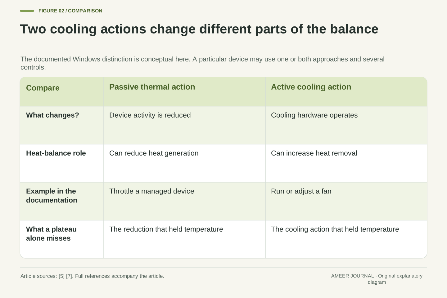
A laptop finishes the first part of a long task quickly, then makes slower progress while its reported temperature barely changes. The flat temperature line does not rule out a thermal constraint. A controller can reduce heat production as the system approaches a target, leaving temperature steady because less heat is entering. Windows documents this kind of performance reduction as passive cooling, distinct from active cooling such as running a fan. [5] Both approaches can influence the same temperature record through different actions.

That explanation is a possibility to investigate, not a diagnosis from one number. A reported temperature, a power reading and completed work answer different questions. The Linux power allocator documentation provides a concrete example in which temperature helps determine permitted power; Intel describes manufacturer-selected platform policies. [6][7] A stable reading may therefore be an outcome of control. To understand sustained performance, follow what the system was allowed to do over time, as well as how warm one monitored location became.

A temperature plateau does not establish that thermal constraints are inactive. In a controlled system, the manipulated variable can change while the controlled temperature remains near its target. Windows distinguishes passive reduction of device heat generation from active cooling hardware; a specific Linux thermal governor uses temperature feedback to determine power allocation. [5][7] Consequently, a constant temperature and a falling work rate are compatible observations. Neither proves the cause of the other without additional evidence about the workload and controlling constraints.

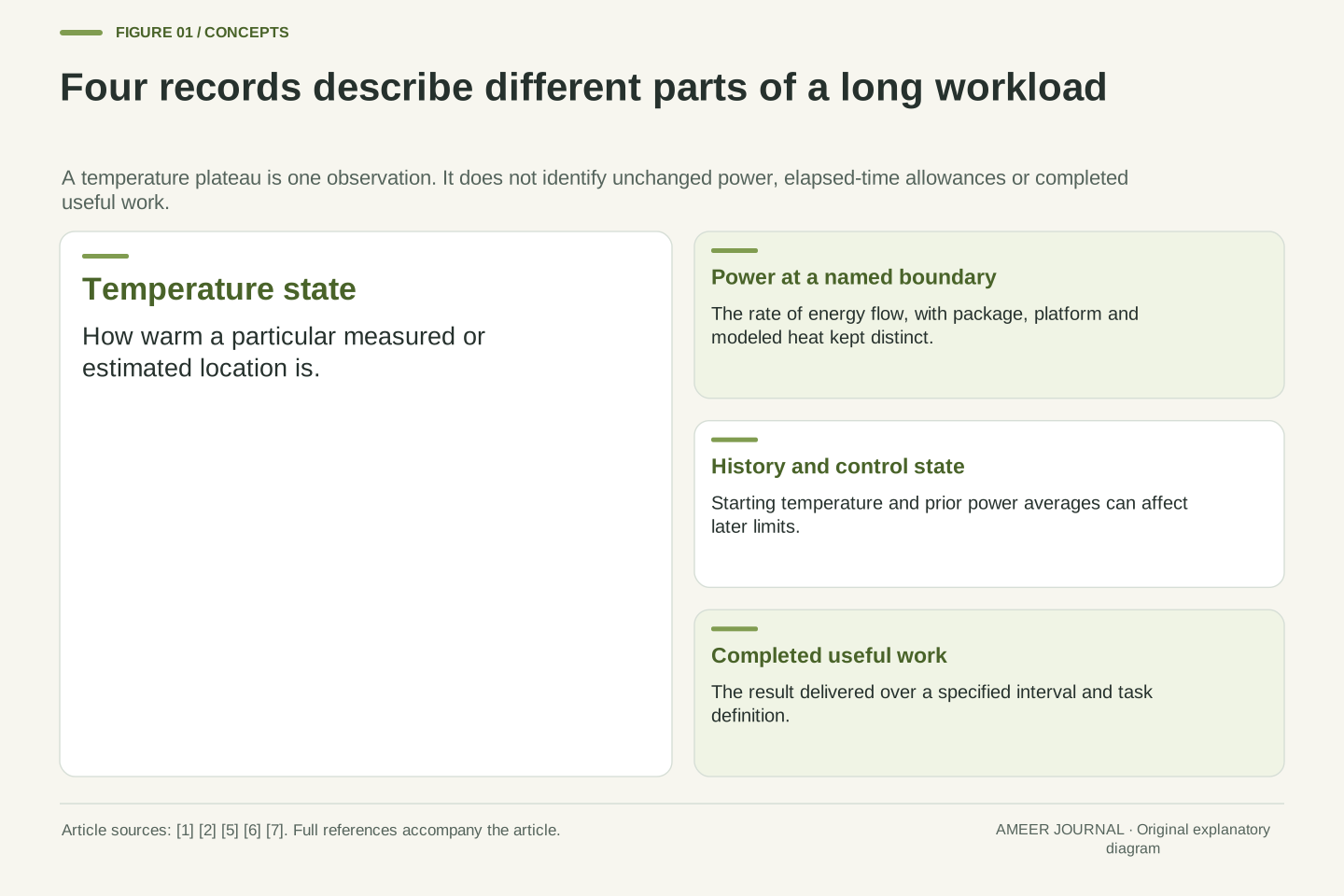
Keep the measured state, control action and useful output separate. A temperature trace describes a sensor or estimated thermal state; a power trace describes energy flow across a named boundary; completed work measures an application result. Intel DTT documents OEM-selected policies that may coordinate platform resources. [6] That is an example of why the relationship need not be a fixed temperature-to-frequency lookup. We will construct two separate analytical models to show what those distinctions allow, without inferring a particular laptop's controller from its external readings.

Imagine one uniformly warm body representing an effective part of a cooling system. It can store thermal energy and release heat to surrounding air. MathWorks documents these as separate properties: thermal mass stores energy, while thermal resistance relates heat flow to a temperature difference. [3][4] Our invented body stores 80 joules for each degree of temperature rise. Its chosen resistance means a difference of one degree drives one watt of heat outward. These properties remain constant throughout the first calculation.

Set the air to 25°C and the body initially to 45°C. Deposit 50 watts of heat in the body and choose 65°C as an illustrative control ceiling. That ceiling is a mathematical choice, not a processor limit or a recommended surface temperature. This single body does not resolve a real laptop's chip, case and internal temperature differences. Its 50 watts mean heat entering this body, not a reading at the wall socket. With that scope established, we can account for incoming heat, outgoing heat and the energy still being stored.

Use a lumped isothermal node with heat capacity C=80 J/K and effective resistance R=1 K/W to a prescribed ambient Ta=25°C. Let P=50 W be heat deposited in that node, with initial state T0=45°C. The constant-mass and resistance relations give C dT/dt=P−(T−Ta)/R. [3][4] Capacity determines the energy associated with a temperature change; resistance determines the heat-flow rate for a given temperature difference. Celsius differences equal kelvin differences here, so no absolute Celsius ratio enters the balance.

Choose an illustrative ceiling L=65°C. All parameters are invented, fixed and positive; the node has no additional heat paths or spatial gradients. It is not identified with a CPU junction, a chassis surface or an entire measured laptop. P is thermal input inside the defined boundary, rather than an assumed synonym for package or wall electrical power. The model supplies an explicit mechanism and checkable units. It does not supply a real product's permitted temperatures, fan curve, thermal material properties or task-completion rate.

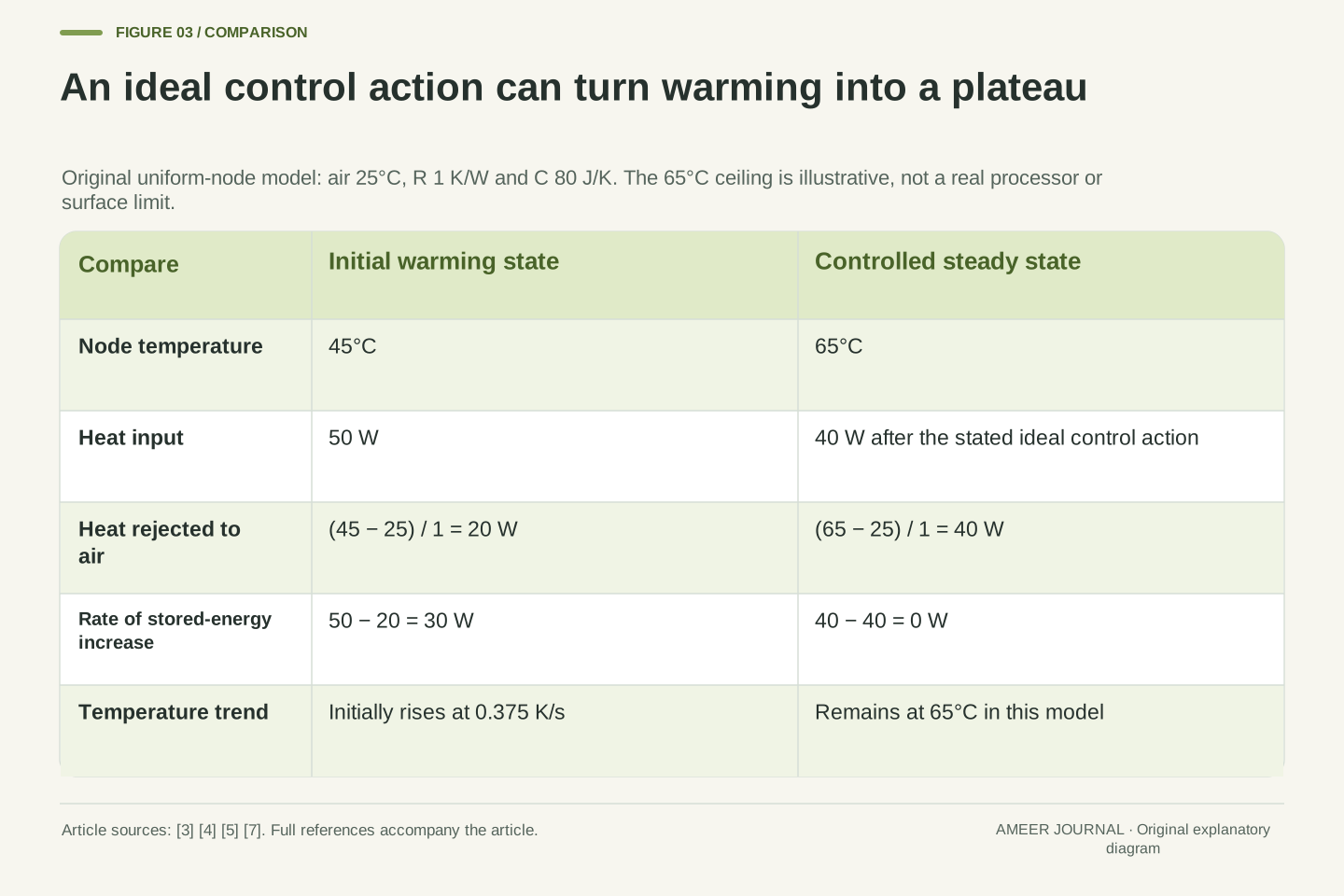
At the start, the body is 20 degrees above the air, so 20 watts leave it. With 50 watts entering, the remaining 30 watts increase its stored energy. As it warms, the temperature difference grows and more heat leaves. The body therefore warms progressively more slowly even though its input stays fixed. This follows from the same storage and resistance relations, not from a changing processor workload. [3][4] If the input continued indefinitely without control, the model would approach 75°C.

The chosen 65°C ceiling is reached after about 87.89 seconds. Raising the body from 45°C to 65°C stores 80 × 20=1,600 joules. By that time, the 50-watt input has delivered about 4,394.45 joules, and about 2,794.45 joules have already escaped to the air. Heat was leaving during the burst; it was simply not leaving as quickly as it arrived. Dividing 1,600 joules by the initial 30-watt surplus would give only 53.33 seconds, because that shortcut wrongly keeps the initial surplus constant as the body warms.

For constant input before any intervention, τth=RC=80 s and the equilibrium is T∞=Ta+PR=75°C. Solving the stated balance gives T(t)=75−30 exp(−t/80). Initially, heat rejection is 20 W and storage rate is 30 W, so dT/dt=0.375 K/s. As T rises, rejection increases and the derivative decreases. [3][4] The unconstrained solution reaches 65°C when exp(−t/80)=1/3, giving t*=80 ln(3)=87.88898 s. This crossing is a property of the fixture, not a measured turbo interval.

The stored-energy increase is C(L−T0)=1,600 J. Total deposited energy is Pt*=4,394.449 J; integrating the outgoing flow gives the remainder, 2,794.449 J. Thus the transient is not an interval of zero cooling. Its energy balance contains both storage and ongoing rejection. Assuming the initial 30 W storage rate persists would predict 53.333 s and violate the temperature-dependent outgoing flow. The distinction matters when interpreting a short run: a device can draw on thermal storage during that interval without demonstrating that the same input is sustainable indefinitely.

Now add an idealized controller to the heat example. At the chosen 65°C ceiling, the body is 40 degrees warmer than the air, so it releases 40 watts. If the controller reduces incoming heat from 50 watts to 40 watts at that moment, incoming and outgoing rates match. Stored energy stops increasing and the temperature stays at 65°C. The plateau is produced by the reduced input; it does not show that the earlier 50-watt state can continue unchanged.

This is a simplified way to understand why a temperature line may flatten while available processing changes. Windows describes reducing device activity as one thermal-management action, and the Linux governor documentation explicitly discusses controlling toward a temperature with an estimated sustainable power. [5][7] Our ideal switch is not either implementation. Nor does a 20% reduction in the model's heat input imply a 20% reduction in useful speed. The calculation establishes a heat balance. A claim about task performance needs its own work measurements.

At T=L=65°C, Qout=(65−25)/1=40 W. Define an ideal controller that changes P from 50 W to 40 W exactly at t*. The subsequent balance becomes C dT/dt=40−40=0, making T=65°C a constant solution. The temperature itself is continuous at the switching moment. This is a constructive example of a thermal constraint with no continuing temperature rise. It also explains why substituting the original 50 W into the later balance would be incorrect: the control action changed the boundary condition.

Real implementations can use several sensors, limits, delays and actuators. The specific Linux power allocator treats sustainable power as an estimate and uses feedback; Windows exposes active and passive thermal-management approaches. [5][7] Those sources support the control distinction, not our instantaneous switching law. The heat-input ratio 40/50=0.8 is therefore not a derived frequency, throughput or battery-runtime ratio. A plateau constrains the thermal balance under the model, while the relationship between permitted power and useful computation remains a separate question.

Double the body's capacity to 160 joules per degree while keeping its resistance, air temperature and starting temperature unchanged. The same 20-degree rise now stores 3,200 joules, and the uncontrolled time to the ceiling doubles to about 175.78 seconds. Yet at 65°C the body still releases only 40 watts. More storage extends this particular burst; it does not raise the steady heat input that the unchanged path can reject at that ceiling. Capacity and thermal resistance are different properties. [3][4]

Changing the path gives a different result. With resistance reduced from 1 to 0.8 degrees per watt, the same 40-degree difference can drive 50 watts outward. In a separate case, raising the air temperature from 25°C to 35°C while retaining the original resistance leaves only a 30-degree difference, allowing 30 watts at the chosen ceiling. These comparisons hold all unmentioned assumptions fixed. They do not say that doubling fan speed halves resistance, or that adding material to a real device changes only its capacity.

Increasing C from 80 to 160 J/K changes τth from 80 to 160 s. The unconstrained crossing becomes 160 ln(3)=175.77797 s, and stored energy to the ceiling becomes 3,200 J. However, the sustainable model input at that ceiling remains Ps=(L−Ta)/R=40 W, independent of C. [3][4] This separates transient storage from steady rejection. A larger capacity changes the trajectory's time scale; it does not alter the equilibrium relation when all other parameters are held fixed.

By contrast, R=0.8 K/W gives Ps=50 W at the same L and Ta. A 50-watt run beginning below the ceiling then approaches 65°C asymptotically in this fixed model. Separately, Ta=35°C with R=1 K/W gives Ps=30 W. These are parameter sensitivities, not predictions for particular fans or enclosures. An actual change can affect several paths and capacities simultaneously. The relevant physical inference is narrower: changing resistance or ambient conditions changes the allowable steady heat-flow balance, whereas changing capacity alone does not.

Heat is not the only quantity a platform may control. Intel's 12th-generation processor datasheet, revision 011, describes PL1 as an average-power threshold and PL2 as a separate threshold addressed by rapid power-limiting algorithms. It describes Tau as an averaging constant used in the PL1 calculation. [1] These are named controls in that documentation, rather than universal labels for every laptop. A manufacturer's configured limits and policies belong to the particular system being examined.

The same datasheet explains that a maximum-power turbo event can remain at PL2 for longer than the numerical Tau value. [2] That directly undermines the idea that a parameter labelled in seconds must mean a fixed boost countdown. An average can depend on earlier activity, and other constraints can act before or during a run. Treat a documented time parameter according to its definition. Do not substitute it for the thermal time constant in our heat equation, or infer an exact task duration merely because both quantities use seconds.

In Intel document 655258, revision 011, PL1 constrains average power, PL2 has a distinct rapid limiting role, and Tau participates in the PL1 exponentially weighted moving-average calculation. The page also describes separate PL3 and PL4 mechanisms. [1] This is a scoped processor-family example of multiple controls, not an assertion that every system has one immutable power budget or uses these names. Platform configuration and dynamic policies can affect the operating limits described in that documentation.

The associated Tau section expressly permits a maximum-power turbo event to sustain PL2 longer than Tau and notes settling after runtime parameter changes. [2] Therefore Tau cannot be interpreted as a universally enforced residence time at PL2. It has the dimension of time but belongs to an algorithmic state calculation. The physical τth=RC belongs to our thermal differential equation. Equal units do not identify the two quantities, and neither parameter by itself determines a workload's useful completion time or which constraint acts first.

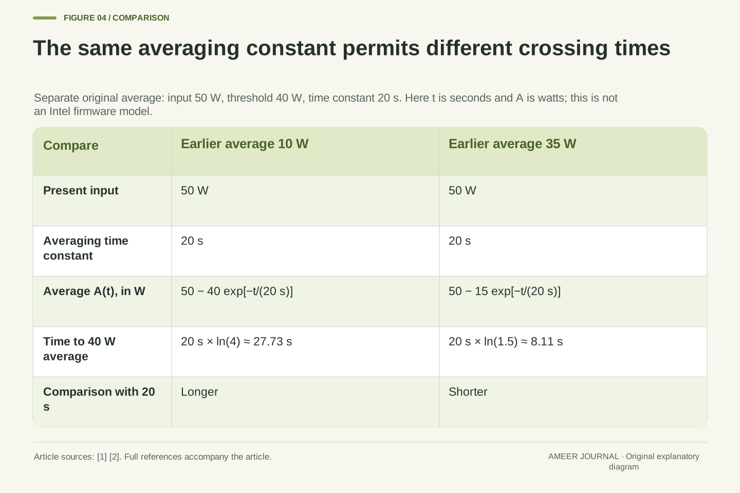
To see how prior activity matters, make a separate mathematical example. Let the present power be a constant 50 watts, and let a smoothed power record move gradually toward it with a 20-second averaging time. Choose a threshold of 40 watts for that smoothed record. If its starting value is 10 watts, it reaches 40 watts after about 27.73 seconds. The instantaneous input was already 50 watts; it is the separate average that is catching up. This record has units of watts, not degrees.

Start the smoothed record at 35 watts instead, with everything else unchanged, and it reaches the same threshold after about 8.11 seconds. One result is longer than 20 seconds and the other is shorter. The averaging time did not change; the earlier state did. Intel's documentation supplies the reason to distinguish an average and its parameter from a fixed duration. [1][2] Our continuous calculation merely illustrates that distinction. It is not a reconstruction of Intel's controller or a prediction that a particular laptop will boost for either interval.

Define a separate illustrative state A with dA/dt=(P−A)/τp, P=50 W and τp=20 s. For a constant input, A(t)=50+(A0−50)exp(−t/20). Set the illustrative average threshold to 40 W. With A0=10 W, the crossing satisfies exp(−t/20)=1/4, so t=20 ln(4)=27.72589 s. This is a continuous first-order averaging model that retains prior-state information with exponential weighting. It illustrates the distinction in the Intel documentation; it is not a disclosed implementation of its microcode. [1][2]

For A0=35 W, the same threshold requires exp(−t/20)=2/3, giving t=20 ln(1.5)=8.10930 s. Both cases have identical present power, threshold and averaging constant. Their history-dependent initial averages produce different crossing times. A is a power state measured in watts, not a temperature measured in degrees. The example demonstrates why reading a time constant as an elapsed-time allowance discards necessary state information. It does not supply the response of any additional power, current, thermal or platform constraint.

The physical heat example has its own history. Starting its body at 60°C instead of 45°C leaves less room below the chosen 65°C ceiling. With the same 50-watt input and original capacity and resistance, the calculated crossing falls from about 87.89 seconds to about 32.44 seconds. The hardware parameters in the model did not change. Only the starting temperature did. A run begun after earlier activity therefore need not follow the same transient as a run with a different initial thermal state.

Keep that comparison separate from the smoothed-power example. One state describes stored heat; the other remembers power history. If a real control reduces power, the earlier equation that assumed a constant input must change. [1][2][3][4] You cannot let both uncontrolled curves continue unchanged after one constraint has already altered the input. Comparing their example crossing times is not a simulation of a complete laptop. It shows which starting states and control events would have to be known before such a simulation could make a defensible prediction.

With the original thermal parameters but T0=60°C, the unconstrained trajectory is T(t)=75−15 exp(−t/80). Its 65°C crossing is 80 ln(1.5)=32.43721 s, compared with 80 ln(3)=87.88898 s from 45°C. This initial-condition sensitivity follows from the heat balance. [3][4] It is independent of whether a policy average A begins at 10 or 35 W. Physical temperature and filtered power carry different information even when both reflect activity before the chosen start time.

Do not merge the separate constant-input examples into an unstated coupled simulation. An earlier control action changes P(t), after which both the thermal balance and any power-average state must be advanced using the changed input. Intel's runtime-limit discussion reinforces the need to account for state and settling rather than treating all limits as simple timers. [1][2] Our 80-second thermal constant and 20-second illustrative policy constant are therefore neither interchangeable nor additive boost allowances. The calculations identify required state variables, not an actual device's first limiting event.

A laptop also contains more than one source of heat. Intel's DTT description discusses finite platform resources shared across components, while Windows describes coordinated thermal zones. [5][6] Those descriptions do not imply that every CPU and GPU has one common sensor or an identical heat path. They do show why an application's available CPU power should not be inferred from a temperature reading without considering what other parts of the platform are doing.

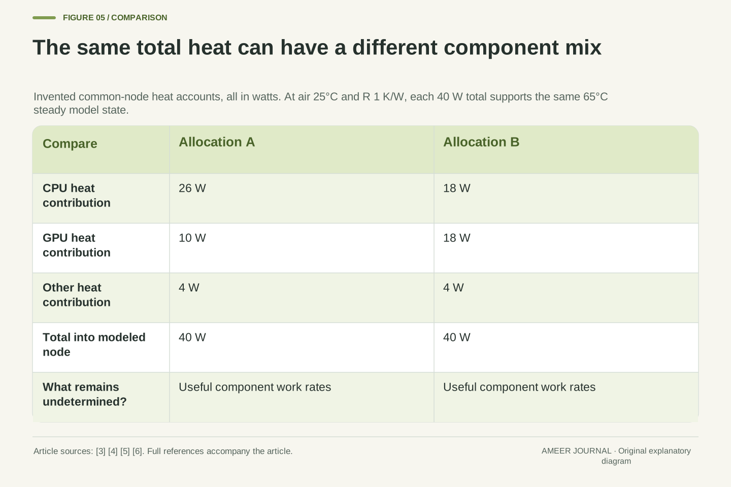
Return to our single-body example solely for an invented allocation. At the 65°C ceiling, its 40-watt heat budget could contain 26 watts from a CPU, 10 from a GPU and 4 from other sources. Another allocation could be 18, 18 and 4 watts. Both total 40 watts, so both can maintain the same model temperature. The CPU's share fell while the GPU's rose. These numbers are heat contributions inside the same assumed boundary, not real processor specifications. They establish neither component's useful work rate.

Platform coordination can allocate resources among multiple devices, as illustrated by the Windows thermal-zone model and Intel's DTT documentation. [5][6] The actual physical topology and policy remain system-dependent. A package power domain, a thermal zone and an application's resource demand should not automatically be treated as identical sets. The Linux governor documentation likewise requires consistent power scales among devices participating in a zone. [7] A common numerical budget is meaningful only after its boundaries and units have been defined.

For a deliberately simplified common-node allocation, define all contributions as heat entering our node. Case A has CPU/GPU/other contributions of 26/10/4 W; case B has 18/18/4 W. Each sums to 40 W, matching rejection at 65°C with Ta=25°C and R=1 K/W. The same steady temperature thus permits different component allocations. This is an accounting counterexample to inferring an unchanged CPU share from unchanged temperature. It does not claim a real laptop has one isothermal CPU/GPU body, or that either allocation determines a proportional application-speed change.

A power number needs to say where it was measured. Heat entering our invented body, electrical power reported for a processor package and consumption measured for a whole laptop are different records. Active cooling itself consumes power, and Windows includes devices such as charging hardware among possible thermal-management participants. [5] A whole-system change can therefore involve energy use outside the processor activity you were watching. It should not silently become the 50 watts in our thermal example.

For instance, energy stored in a charging battery is not automatically heat deposited in the chosen cooling body. A fan's electrical consumption is also a separate item unless the model explicitly accounts for where that energy goes. The same discipline applies to time: a momentary reading is not the energy used over a complete task. To compare runs, keep the measurement boundary and interval consistent. A steady temperature alone gives no total electrical-energy result, and a larger whole-system reading alone does not identify how much additional heat reached one sensor's surroundings.

The model input P has a thermal boundary definition. Replacing it with a package electrical reading or whole-system electrical input requires an explicit energy balance that accounts for storage and other destinations. Windows documents active-cooling power consumption and management of devices beyond the processor; Intel distinguishes package control from broader platform policy. [1][5][6] These descriptions support keeping those domains separate. Our one-node equation has not established a conversion from any particular telemetry field to net heat deposited in that node.

Similarly, energy is the time integral of power at the selected boundary, not a temperature plateau or an isolated maximum reading. Battery charging can store energy outside the modeled body, and fan power belongs to a declared boundary rather than an assumed zero-cost cooling action. Two runs with equal node temperature can therefore have different electrical-energy accounts. This is a conservation and measurement-definition issue, not a claim about the efficiency of a specific adapter, battery or fan. Preserve the distinction when reading both instantaneous values and task-level totals.

To discuss useful speed, define the work being counted. Consider an invented log of identical work units: the first 30 seconds complete 8 units per second, while the next 270 seconds complete 5 units per second. The first part completes 240 units and the second completes 1,350, for 1,590 units over 300 seconds. The whole-run average is therefore 5.3 units per second. Extending the initial rate across all 300 seconds would predict 2,400 units, which this log does not deliver.

A plain average of the two rates would also be wrong: 8 and 5 average to 6.5, but the slower interval lasts nine times as long. Neither rate was calculated from our thermal example; they are separate invented observations used to explain measurement. Thermal management can affect device performance, but its effect on an application needs the application's own result. [5] Keep the short interval if responsiveness matters, and report the complete interval when discussing sustained work. Their different answers can both be accurate when their windows are stated.

Use a defined work unit and a matching observation interval. In an independent hypothetical log, let r=8 units/s for 30 s and r=5 units/s for the following 270 s. Each interval counts the same stipulated work unit. Integrated work is 8×30+5×270=1,590 units, giving mean throughput 1,590/300=5.3 units/s. The unweighted mean of the two rates, 6.5 units/s, ignores unequal durations. Extrapolating the first interval instead yields 2,400 units, a different prediction from the defined log.

This work record is not derived from the 50-to-40-watt thermal transition. A relationship between heat input, electrical power, frequency and application throughput would require additional workload and system evidence. Windows' performance-scaling description does not establish a universal linear mapping between those quantities. [5] Report startup or burst performance and sustained throughput as separate metrics when both matter. The work unit, task correctness, interval and initial state are part of the definition; an isolated peak frequency is not a substitute for that result.

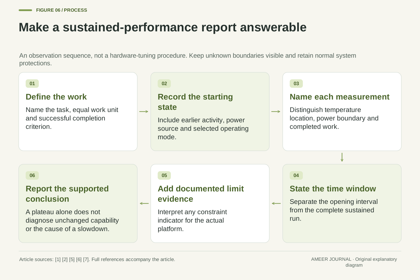
A useful comparison names the task, the identical work unit or completion criterion, the starting conditions, power source, selected operating mode and the time window. Record temperature, relevant power readings and completed work as separate signals. Where available, add the system's own indication of an active constraint and identify what it means for that platform. Intel's manufacturer-defined tuning and Windows' coordinated thermal management make that context relevant. [5][6] Unknown sensor locations or power boundaries should remain explicitly unknown.

Then describe the observation before assigning a cause: perhaps the work rate fell, a package-power reading fell and a particular temperature became steady during the same interval. That is stronger evidence than the temperature alone, but a causal conclusion still needs the relevant control and workload information. The examples here explain why the combination is possible. They also explain why a fast first interval, a cool starting state or a flat later temperature cannot by itself establish sustained capability. Keep normal protections intact and use the actual system's documentation to interpret its records.

A reproducible run record binds workload identity and correctness, start/history, power source and mode, measurement boundaries, sampling semantics and interval length. Log the relevant temperature state, electrical or thermal power quantity and useful work separately. If the platform exposes constraint indicators, interpret them according to the applicable documentation rather than treating a familiar label as universal. Intel's scoped control descriptions and OEM policy selection, together with Windows' platform coordination, explain why these fields matter. [1][2][5][6]

The final inference should match the record. A temperature plateau alone does not identify the controller, establish unchanged power allocation or prove a fault. Our thermal example shows a plateau created by lower input; the averaging example shows a state-dependent threshold time; the work log shows why a short rate cannot represent every longer interval. Combining those distinctions makes a slowdown report testable without pretending that one analytical fixture is a laptop benchmark. Retain the original system controls and seek the missing workload or limit evidence before attributing the observed change to a specific mechanism.