What you’ll take away
- Identify whether a number is a filter factor, stop count, optical density or transmitted percentage before calculating.
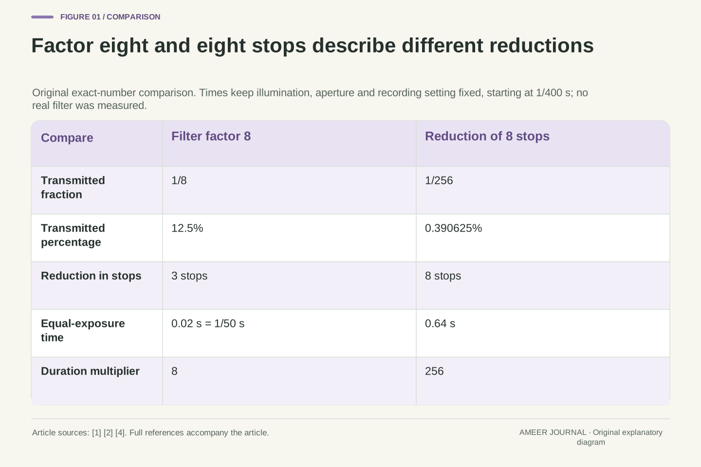
- A factor of eight means three stops and one eighth transmission; eight stops instead means a factor of 256.
- For ideal scalar stacks, factors multiply while stops and optical densities add.
- Nominal labels, wavelength conditions and tolerance quantities must stay separate from exact mathematical examples.
- A variable control needs its own calibration; equal rotation angles need not give equal changes in stops.
The number needs a scale before it can describe the reduction
An ND filter reduces light reaching the camera, but the number beside its name needs interpretation. In Nikon's published chart, ND8 appears in the filter-factor column and corresponds to three stops and 12.5% transmission [2]. The eight describes a ratio: one eighth of the original light passes through under the stated comparison. Three stops describes the same reduction through three successive halvings. Treating that factor as eight stops would describe a much stronger reduction, so the distinction affects an exposure calculation immediately.
The useful first question is therefore what the number measures. A specification might give a factor, a stop count, a transmission percentage or optical density, which is another numerical scale [1][2][4]. We will translate among them using original paper examples. The models keep illumination and camera settings fixed unless a change is explicitly stated. They describe optical transmission and exposure, not a test of a particular filter or a guarantee about a finished photograph's appearance. A separate ideal-polarizer example will show why a rotating control also needs its own interpretation.
An ND specification can express attenuation using several dimensionless quantities. Nikon's chart explicitly labels ND8 as a factor entry corresponding to three stops and 12.5% transmission [2]. A factor of eight means transmitted optical intensity is one eighth of the reference intensity under the specified conditions. An eight-stop reduction instead has factor 256. The integer alone therefore cannot identify the physical transmission until the reporting convention is known.
The analysis below uses original scalar transmission and linear optical-integration examples, followed by explicitly separate spectral, tolerance and ideal-polarizer cases. Conditions such as input spectrum, polarization, angle of incidence and spatial uniformity matter to the definition of a transmission [1][4][6]. No product was measured. The objective is to preserve the quantity and its reference while moving among notation systems, rather than treating a convenient photographic label as an independently calibrated value or a rendered-image brightness measurement.
Start with the fraction that actually passes through
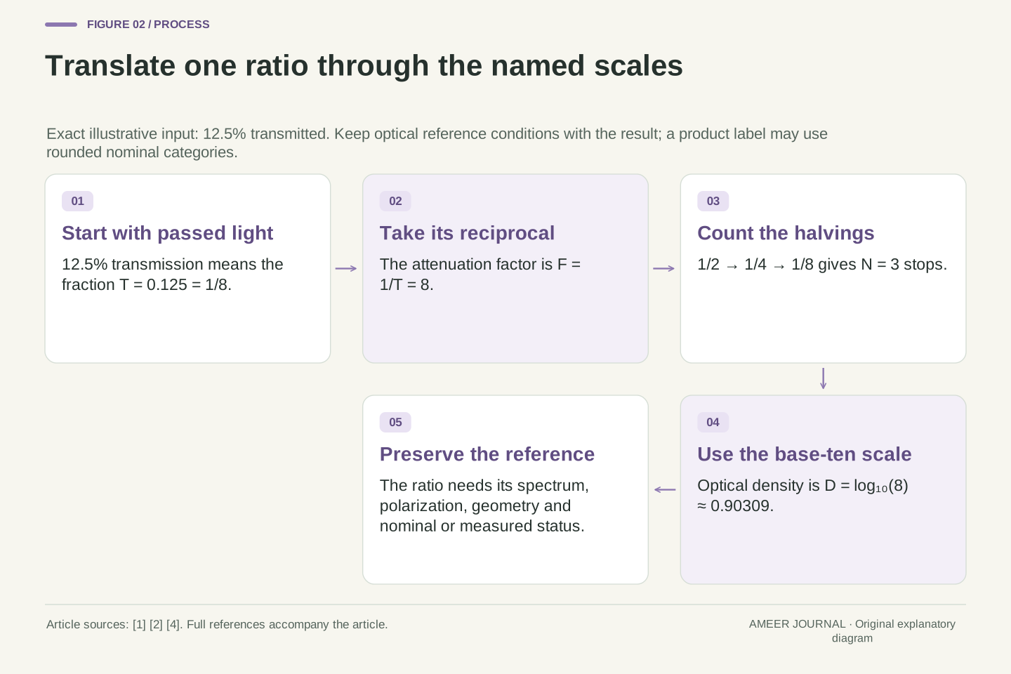
Transmission tells us how much light passes through compared with the light arriving, using the same measurement conditions. Write that fraction as T. If 12.5 units pass for every 100 units arriving, T is 0.125 and the transmitted percentage is 12.5%. The remaining 87.5% does not pass through in that comparison. This is different from saying that the filter blocks 12.5%. Edmund Optics and Newport express density through transmitted light, so keeping the passed amount clear prevents the calculation from starting with the wrong fraction [1][4].
The quantity also needs a context. Are we describing the whole stated wavelength band, a particular wavelength or one defined input condition? A percentage is useful only when the numerator and reference are comparable. Nor is it a direct reading of how bright the preview looks. If a camera changes another exposure setting after the filter is fitted, the resulting image can change for more than one reason. Our simple calculations keep those other choices fixed so that the filter's optical contribution can be followed on its own.
Define fractional transmittance T as transmitted divided by incident optical intensity for the specified optical conditions, with 0<T≤1 in the logarithmic examples. Percent transmission is 100T. Thus T=0.125 means 12.5% transmitted and 87.5% not transmitted. These quantities must not be exchanged. The retained application notes define optical density through transmittance, although one writes T as a percentage and the other as a fraction [1][4]. Explicitly normalizing that convention avoids an erroneous factor of 100 inside a logarithm.
This is an intensity or energy relation, not an electric-field-amplitude relation. The reference must preserve the relevant spectral, polarization and geometric conditions; those assumptions become visible in the later examples. A display value or processed pixel code is another quantity with additional operations between incident light and appearance. Consequently, observing similar preview brightness before and after adding a filter would not alone establish T. The exposure comparison must identify which settings and optical inputs remained unchanged and which were adjusted.
Factor, stops and optical density encode the same ratio differently
A filter factor is the reciprocal of transmission. If T is 1/8, the factor is 8. Each full stop of reduction halves the transmitted amount, so the sequence is one half, one quarter, then one eighth: three stops. Eight stops would continue that halving process to 1/256, which is only 0.390625% transmission. These are mathematical conversions of stated inputs. The ND8 entry in Nikon's chart follows the factor convention; checking the column heading is what makes its number useful [2].
Optical density uses powers of ten instead of repeated powers of two. Edmund and Newport give the corresponding transmission relationship [1][4]. A density of 1 means 10% transmission; a density of 2 means 1%. For exact factor 8, optical density is about 0.90309. That decimal, the factor 8, three stops and 12.5% transmission can all describe the same ideal reduction. They are different names for related quantities, not four separate effects to add together. A reliable explanation keeps the name attached whenever it quotes the number.
Let F=1/T be attenuation factor, N=log₂F the reduction in stops, and D=log₁₀F the optical density. Then T=2⁻ᴺ=10⁻ᴰ and D=Nlog₁₀2. The density relationship is documented by both optical manufacturers, while Nikon's chart illustrates the photographic factor/stop convention [1][2][4]. All logarithm arguments here are dimensionless ratios. The base matters: a unit change in D is a tenfold intensity ratio, whereas a unit change in N is a twofold ratio.
For T=1/8, F=8, N=3 and D≈0.903089987. For N=8, F=256 and T=1/256=0.00390625. The latter passes 3.125% as much light as the factor-eight case, a ratio of 1/32 between the two transmissions. This is why assigning the same interpretation to every visible integer creates a large error. The conversion framework applies after the specification's quantity is identified; it does not create a universal meaning for an otherwise unexplained product label.
A nominal label and an exact calculation have different precision
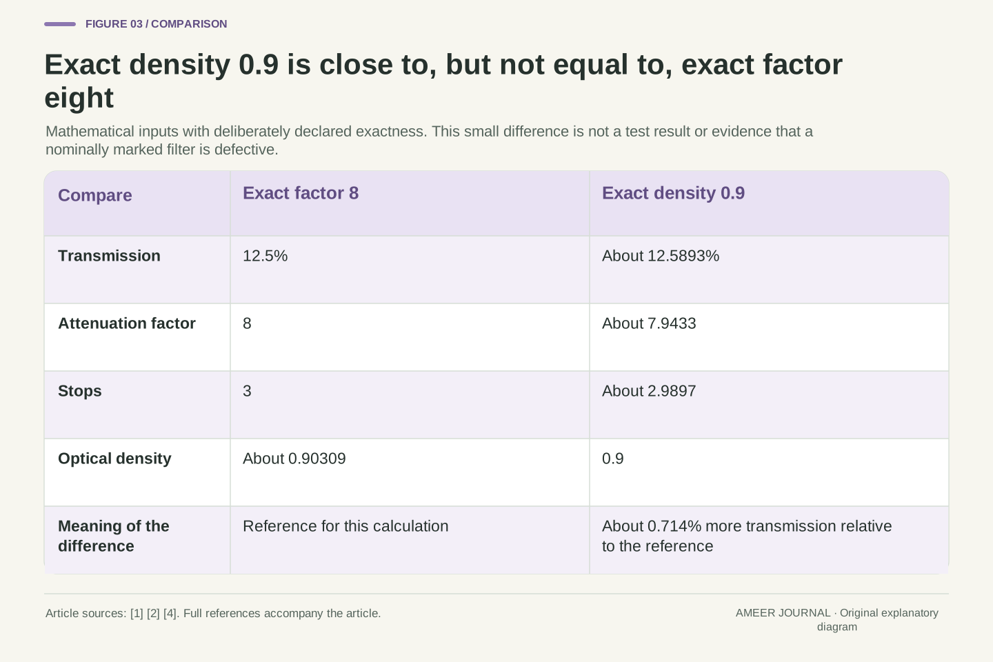
Now suppose a mathematical example declares optical density to be exactly 0.9. Its transmission is about 12.5893%, and its factor is about 7.9433. Exact factor 8 instead means 12.5% and density about 0.90309. The difference in transmitted amount is about 0.714% relative to the exact factor-eight value. The numbers are close, but they are not identical. This comparison follows the density equation [1][4]; it is not a measurement showing that a filter marked 0.9 performs incorrectly.
Photographic charts can use convenient nominal categories. Nikon's same chart pairs ND1000 with ten stops and 0.1% transmission [2], whereas ten exact halvings give factor 1024. That is a reason to read the precision and conditions of a specification before treating every displayed category as an exact identity. A small difference between a calculated value and a rounded label does not by itself establish a manufacturing fault. To assess a real part, one would also need its stated tolerance, reference conditions and suitable measurement evidence.
Using D=0.9 as an exact mathematical input gives T=10⁻⁰·⁹≈0.125892541, F≈7.943282347 and N≈2.989735285. Using F=8 exactly instead gives D≈0.903089987. Their relative transmission difference is (0.125892541/0.125−1)×100%≈0.714033%. This distinguishes arithmetic precision from a product's nominal marking. Neither input represents measured manufacturing variation, and the discrepancy is not an inferred tolerance [1][4].
The Nikon chart itself provides a useful precision check: its ND1000/ten-stop category cannot be an exact equality because 2¹⁰=1024, while log₂1000≈9.965784 [2]. A chart can remain useful as photographic guidance without every displayed value having calibration-grade precision. Preserve whether a number is nominal, rounded, exact by definition or measured. Those statuses determine what a numerical comparison can establish, especially when a specification separately supplies a density tolerance and wavelength condition [4].
Convert the attenuation into time only after fixing the other inputs
Take an original ideal example with a reference exposure of 1/400 second. Hold the scene illumination, aperture and recording setting unchanged. A factor-eight filter passes one eighth as much light per unit time, so an eight-times-longer interval restores the same optical exposure: 8×1/400 second is 1/50 second, or 0.02 second. This is the mechanism behind using ND attenuation to permit a longer exposure while retaining other chosen settings [2][5]. It does not require an ND filter always to be used that way.
The wrong scale produces a visibly different calculation. If the factor 8 were mistakenly treated as eight stops, the duration multiplier would be 256, producing 0.64 second from the same reference. That is 32 times longer than the intended 0.02 second. The example uses exact model durations, not a claim that every camera offers those exact menu values. If the illumination or aperture changes too, the original reference must be updated. A useful exposure calculation records those assumptions instead of applying a memorized multiplier to a different situation.
Under fixed illumination and aperture with linear optical integration, let H₀ be the reference exposure accumulated over t₀. Adding a uniform scalar transmittance T gives H/H₀=Tt/t₀. Equal exposure therefore requires t=t₀/T=Ft₀. This formalizes the photographic use described by Nikon while keeping the optical amount separate from subsequent rendering [2][5]. For t₀=1/400 s and T=1/8, t=1/50 s=0.02 s.
Misreading F=8 as N=8 would instead use t=256/400 s=0.64 s, a factor 32 longer. The arithmetic illustrates a notation error, not a camera experiment. The equality also requires unchanged relevant inputs; automatic changes to aperture or other exposure controls would alter the comparison. Retaining the reference frame's conditions matters as much as applying the exponent correctly. Equal integrated optical exposure in this model does not imply equal motion rendering, since the duration of integration has deliberately changed [2].
Multiply transmission factors while adding stops or densities
For an ideal stack, suppose one neutral filter passes one eighth of the arriving light and a second passes one quarter of what reaches it. Together they pass 1/8×1/4, or 1/32. Their factors multiply to 8×4=32; adding 8+4 would give the wrong answer. The stop counts add instead: three stops plus two stops is five. Optical densities also add, as both Edmund and Newport explain [1][4]. The different arithmetic follows from the scale used to report the same serial reduction.
With our 1/400-second reference, exact factor 32 would require 0.08 second to retain equal optical exposure. That result establishes an attenuation calculation, not whether two physical filters fit the lens or behave as an ideal pair. It assumes each stated transmission applies to the light actually arriving at that element. Later, the polarizer example changes that input state deliberately. Physical mounts, extra reflections and uneven image coverage require their own consideration; they cannot be settled by correctly adding two stop counts [4][5].
For two scalar transmissions under matched conditions, T_total=T₁T₂, F_total=F₁F₂, N_total=N₁+N₂ and D_total=D₁+D₂. Logarithms convert the transmission product into sums in the two logarithmic scales [1][4]. The original T₁=1/8 and T₂=1/4 example gives T_total=1/32, F_total=32, N_total=5 and D_total≈1.505149978. The factor sum 12 has no role in that serial attenuation result.
At t₀=0.0025 s, the corresponding equal-exposure duration is 0.08 s. Each scalar transmission must remain applicable to its actual incident light, and interactions omitted by the model cannot be silently absorbed into the label. Polarization-dependent elements make this condition especially explicit: the first element can alter the state presented to the second [6]. Real stacks may also introduce reflections or vignetting [4][5]. The mathematics therefore describes a declared optical cascade; it does not certify mechanical compatibility, full-field uniformity or actual image quality.
Uniform attenuation preserves a linear highlight-to-shadow ratio
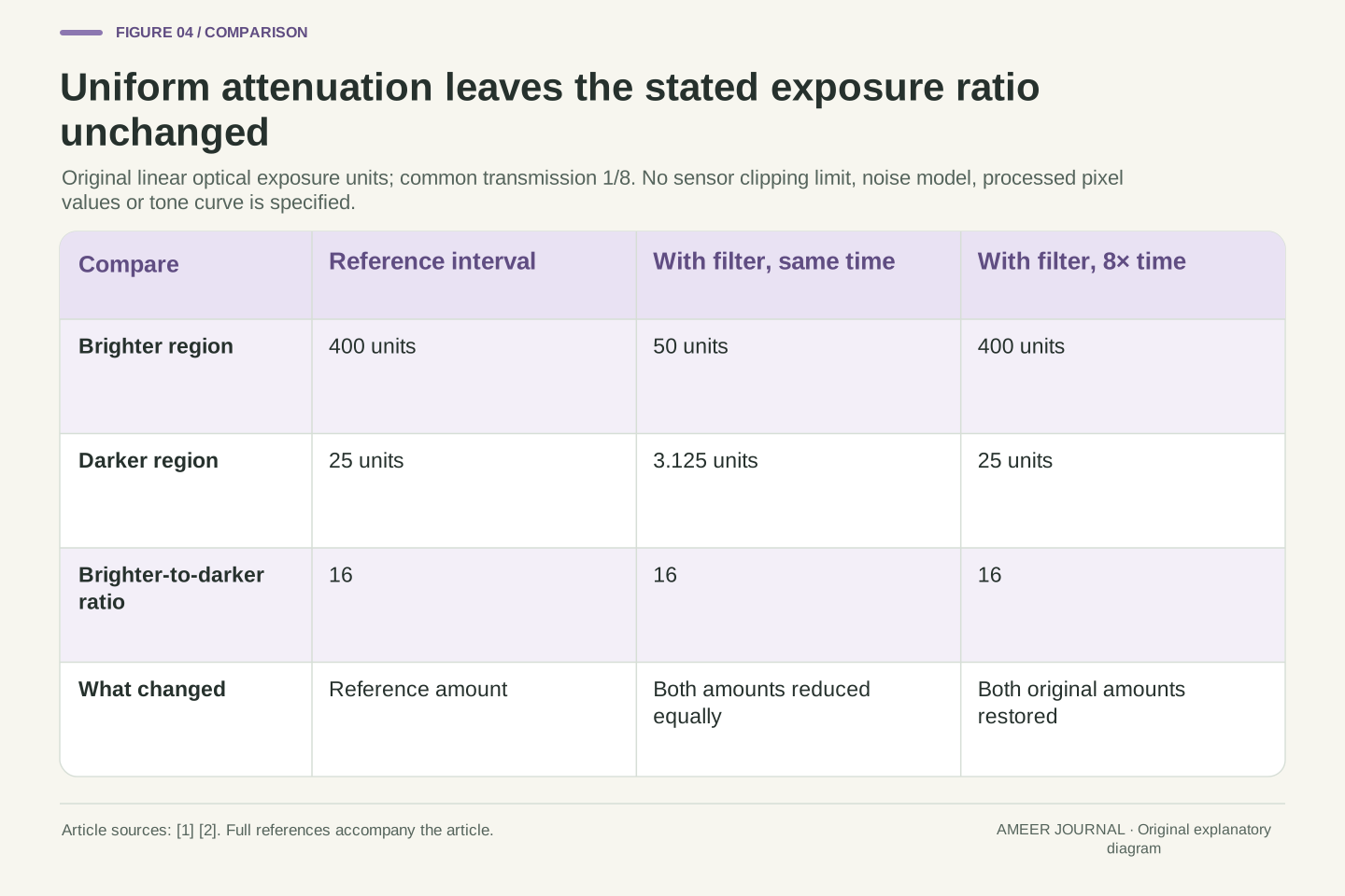
Imagine two parts of a scene that would contribute 400 and 25 arbitrary exposure units during the reference interval. Their ratio is 16 to 1. An ideal filter with transmission 1/8 changes those amounts to 50 and 3.125. The ratio is still 16 to 1 because both numbers were multiplied by the same fraction. These are original linear optical quantities, not camera pixel codes. The deduction follows directly from a uniform transmission applied to both parts of the image [1].
If the interval is then extended eightfold under unchanged light, the two amounts return to 400 and 25, and their ratio remains 16 to 1. Uniform attenuation can change the total amount arriving during a selected interval without compressing that underlying ratio. A spatially varying filter would be a different model, because it would apply different fractions to different image regions. Similarly, a processed preview can include other changes. Keeping the optical ratio separate helps explain why a darker overall image does not automatically mean that a difficult brightness range has been reduced.
For positive linear exposures H_a and H_b with one spatially uniform scalar transmittance T, the ratio after filtering is (TH_a)/(TH_b)=H_a/H_b. In the original case H_a=400 and H_b=25 arbitrary exposure units, T=1/8 gives 50 and 3.125 while preserving the ratio 16. The equation assumes the same effective transmission for both sampled regions. It is an original consequence of the optical-transmission model, not a measured camera dynamic-range result [1].
Multiplying the common integration interval by eight restores both exposure amounts in this ideal stationary-light case and still leaves their ratio unchanged. This distinguishes attenuation from compression of a scene's linear exposure ratio. Spatial graduation, spectrum-dependent transmission and image processing would add different transformations and require different assumptions. The example supplies no detector saturation limit, noise model or tone curve. Its limited conclusion is nevertheless useful: a common positive multiplier cannot by itself change a ratio between two quantities receiving that same multiplier.
Neutrality belongs to a wavelength range and an input condition
Neutral does not mean that a single number describes every possible wavelength. Edmund describes ND attenuation over a specified part of the spectrum [1]. Newport's retained FSR-OD50 page supplies a density at 546.1 nm, a stated range and a transmission curve [4]. The named part is an example of how conditions belong with a specification; its values are not transferred to a photographic filter. A broad statement about darkness leaves out information about which light is being reduced and by how much.
For a separate two-band example, suppose each band would contribute 100 exposure units over the same reference interval. Give the filter 10% transmission in band A and 12% in band B. The outputs become 10 and 12, so the band-B-to-band-A ratio changes from 1 to 1.2. Extending the interval tenfold produces 100 and 120, preserving that changed ratio. A common time adjustment cannot remove this unequal attenuation. This is a simple spectral accounting example, not a camera RGB calculation, a measured colour cast or a promise that one editing adjustment can restore a real photograph.
A real spectral transmission is better represented as T (λ) when wavelength dependence matters. Edmund's scope is explicitly a portion of the spectrum, and Newport's specified part identifies a reference wavelength and transmission-curve context [1][4]. Thus an OD quoted at one wavelength is not, by itself, a complete broadband characterization. The article uses that specification structure as evidence about scope, without claiming the laboratory part is a photographic recommendation or that its tolerance applies elsewhere.
In the original two-band model, equal reference exposures 100/100 become 10/12 under T_A=0.10 and T_B=0.12. Their ratio becomes 1.2. A common tenfold duration multiplier gives 100/120 and cannot restore the original ratio. The inputs here are band-integrated optical exposure units with transmissions stipulated constant within each band. They are not a sensor's overlapping RGB sensitivities or a perceptual colour metric. The calculation isolates why one scalar density cannot fully describe unequal spectral attenuation and why changing time alone does not reverse it.
A density bound becomes an asymmetric transmission interval
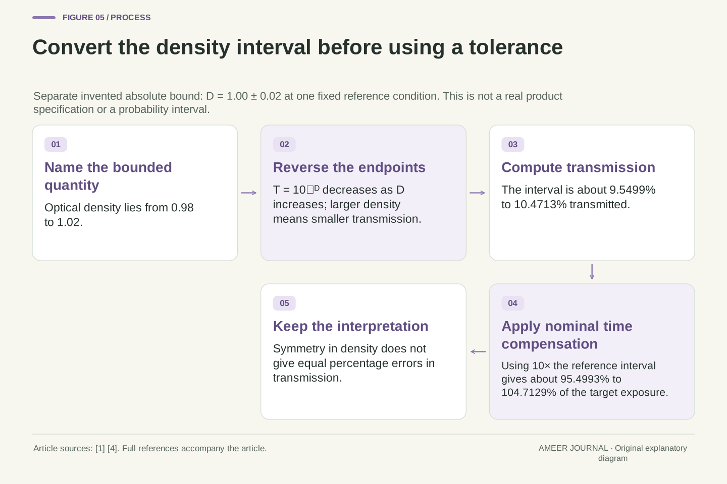
A tolerance must identify the quantity it limits. Newport's specification, for example, labels an optical-density tolerance and includes a reference wavelength [4]. For our own separate illustration, assume density 1.00 with an absolute bound of 0.02 in either direction under one fixed reference condition. Density could therefore lie from 0.98 to 1.02. This is an invented bound, not the tolerance of the Newport part. Applying the density relationship gives transmission from about 9.55% to 10.47% [1][4].
The higher density produces the lower transmission, so the endpoints reverse order when we convert them. If we extend time by the nominal factor 10, the final optical exposure could be about 95.50% to 104.71% of the intended reference under these assumptions. That interval is not exactly symmetric around 100%, even though the assumed density interval is symmetric around 1.00. It is also not a probability or confidence level. The example shows why a tolerance in one numerical scale cannot simply be copied unchanged into another.
Let the separate stipulated bound be D=1.00±0.02 OD at one fixed optical reference condition. This is an absolute density interval [0.98, 1.02], not an actual manufacturer's percentage tolerance. Because T=10⁻ᴰ decreases monotonically, T lies in [10⁻¹·⁰², 10⁻⁰·⁹⁸]≈[0.09549926, 0.10471285]. The logarithmic relation and the need to name the specified tolerance quantity are supported by the retained optical documentation [1][4].
Compensating by the nominal factor 10 gives H/H₀=10T, or approximately [0.9549926, 1.0471285]. Relative errors are therefore about −4.50% and +4.71%, despite the symmetric density input. This is deterministic propagation of an assumed interval; it gives neither a distribution nor a measured performance estimate. It also assumes the stated bound remains applicable to the actual spectrum and optical geometry. A tolerance specified at a different reference condition would need its own justification before entering the same calculation.
A variable control can change the polarization relationship
The instructions for HOYA's named Variable Density II describe two polarized glass elements whose relative rotation changes attenuation [3]. Polarization concerns the direction of light's electric-field oscillation. To understand one simple mechanism, consider two ideal polarizers with initially unpolarized light, meaning the input contains a spread of polarization directions [6]. The first ideal element passes half the original intensity and gives the output a defined polarization. The amount passing the second then depends on its direction relative to that output.
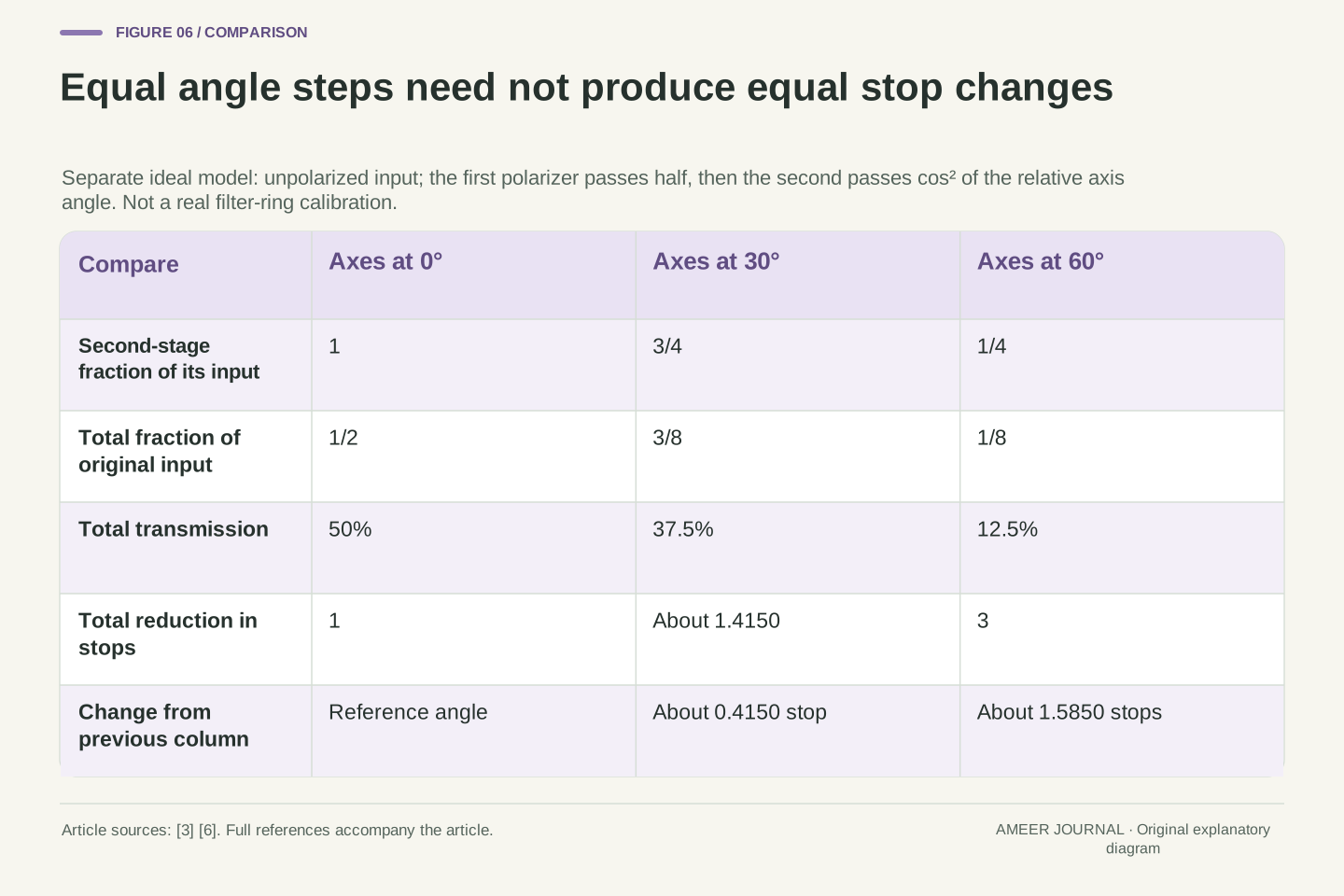
At matching directions, the ideal pair passes half the original light. At a 30-degree separation it passes three eighths, and at 60 degrees it passes one eighth. Those correspond to one stop, about 1.415 stops and three stops. The two equal 30-degree turns therefore produce different changes in stop count. These are original ideal calculations based on the polarization relationship [6], not positions to copy onto a real filter ring. They explain why a rotating control's scale must be established from its documented calibration instead of assumed from equal angular spacing.
HOYA documents two polarized glass elements in its specific Variable Density II [3]. In a separate ideal model, initially unpolarized intensity I_in becomes I_in/2 after the first polarizer. Malus's law then gives I_out=(I_in/2)cos²θ for relative transmission-axis angle θ [6]. The second multiplier applies to already polarized input. Substituting another independent one-half factor for that second stage would lose the state dependence and would incorrectly predict one-quarter transmission even at aligned axes.
At θ=0°, 30°, 60°, the total transmissions from the original input are 1/2, 3/8, 1/8. The corresponding stop reductions are 1, log₂(8/3)≈1.4150375 and 3. Equal 30° increments therefore produce additional reductions of approximately 0.4150 and 1.5850 stops. The model demonstrates nonlinear angular response under explicit assumptions. It is not a calibration of HOYA's mechanism, an assertion about every variable-filter architecture or a calculation of spatial cross-pattern artifacts in a camera image.
Correct attenuation arithmetic does not describe the whole assembly
HOYA's instructions also describe a possible dark cross-shaped pattern near the named filter's maximum attenuation and beyond [3]. That qualification matters when interpreting the product's range. Our ideal two-polarizer numbers do not predict where that pattern appears, what a particular lens sees or how a real ring is marked. A documented limit belongs to the specified assembly and conditions. It should not be replaced with a calculation that assumes perfect components and one uniform ray direction.
Physical stacking brings other questions too. Nikon notes an increased risk of vignetting and image-quality problems when filters are stacked [5], while Newport discusses unwanted reflections from multiple filter surfaces [4]. Vignetting means that part of the image, often toward the edges, becomes darker because coverage or transmission varies. An exact five-stop total says nothing about whether the mount obstructs an image region or whether additional reflections appear. Reading those limits alongside the attenuation scale keeps the calculation connected to the actual optical arrangement.
The named HOYA instructions qualify operation near maximum attenuation with a possible dark cross-pattern artifact [3]. That is source-specific evidence about the assembly, not a result generated by our scalar or ideal-polarizer calculations. A single-angle Malus model lacks the image-field geometry and real component behavior needed to predict the artifact. Its mathematical limiting behavior cannot be promoted into a universal usable range, actual extinction ratio or real-ring calibration.
Likewise, the ideal stack equations omit mechanical obstruction, additional surface reflections and spatial variation. Nikon's stacking discussion identifies vignetting and image-quality risks, while Newport's absorptive-filter account notes unwanted reflections when many elements are stacked [4][5]. These effects can coexist with correctly computed nominal attenuation. Their presence is not resolved by adding density values more precisely. A useful specification separates the scalar amount of attenuation from spectral conditions, assembly compatibility and the spatial behavior that determines whether the whole image receives the assumed transmission.
Keep the number, reference and calibration together
A useful filter record starts with the scale: factor, stops, optical density or transmitted percentage. It then keeps the stated reference conditions, whether the number is nominal or measured, and any tolerance. For a variable model, it also keeps the calibration and the documented usable conditions [1][2][3][4]. Our ideal 30-degree steps made unequal stop changes; the physical ring therefore needs more evidence than its angle alone. The same principle applies to a chart label that rounds several related quantities into a convenient category.
The main example now becomes straightforward. A declared factor 8 means one eighth transmitted and three stops, giving 1/50 second from the unchanged 1/400-second reference. A separate eight-stop reduction means factor 256 and a different result. The stack, spectrum and tolerance examples each changed another assumption, so they should not be mixed into one unexplained multiplier. Read the quantity first, perform the matching conversion, and keep the optical conditions beside the answer. That makes the number useful without asking it to describe every aspect of a finished photograph.
An interpretable attenuation record identifies the quantity, incident reference, spectral and polarization conditions, nominal precision and applicable tolerance [1][4][6]. A variable assembly adds its documented control calibration and range limitations [3]. The ideal angle table is a reminder that equal control increments need not imply equal increments in a logarithmic output quantity. A real relationship between ring position and density must come from suitable documentation or measurement, not the convenience of dividing a circle into equal angles.
For the original fixed-condition case, F=8, N=3 and T=1/8 are mutually consistent, and t=Ft₀ gives 0.02 s. The other examples retain separate assumptions: serial scalar factors multiply, uniform attenuation preserves a positive exposure ratio, spectral imbalance survives common time compensation, and a symmetric density bound becomes an asymmetric transmission interval. Those deductions support a precise reading habit. Preserve the definition and conditions before calculating, then state only what that model or specification actually establishes.
Sources & further reading
Explore the references behind this guide. External pages may change after our review.
- Understanding Neutral Density Filters | Edmund OpticsEdmund Optics · Accessed 7 Nov 2026
- The Joy of Long Exposure PhotographyNikon · Accessed 7 Nov 2026
- HOYA Variable Density II — InstructionHOYA · Accessed 7 Nov 2026
- FSR-OD50 Neutral Density FilterNewport / MKS · Accessed 7 Nov 2026
- A Guide to Lens Filters: How to Improve Your PhotographyNikon · Accessed 7 Nov 2026
- 1.7 Polarization - University Physics Volume 3 | OpenStaxOpenStax / Rice University · Accessed 7 Nov 2026
Article updated 7 Nov 2026.
Found something we should revisit?
Good explanations get better with thoughtful feedback.