What you’ll take away
- A vocabulary table contributes one full learned vector for every declared token identifier.
- In the original example, halving the processing blocks removes about 18% of total parameters because the large table is unchanged.
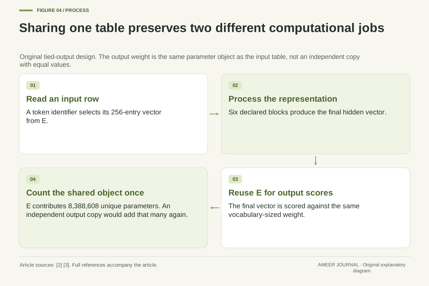
- True input/output weight sharing counts one parameter object even though it serves two computational roles.
- Depth, width and vocabulary size change different terms in a parameter inventory.
- Parameter counts alone do not establish trained quality, token lengths, runtime memory or speed.
A small model can have a surprisingly large vocabulary table
A small language model is often pictured as a short stack of processing layers. That picture misses another substantial component: the table that connects token identifiers with learned vectors. If that table takes a large share of the model’s parameters, removing half the processing layers will remove much less than half the model.
There is a concrete published example. Google’s August 14, 2025 announcement for Gemma 3 270M describes a rounded total of 270 million parameters, split into 170 million embedding parameters and 100 million transformer parameters [1]. Those are the publisher’s rounded figures for that named release, not a universal formula for small models or a current product recommendation.
We will build a separate, deliberately simple parameter inventory to understand the mechanism. It describes an untrained teaching architecture, not Gemma or a usable chatbot. We will count its learned numbers exactly, then change its depth, width, vocabulary and output sharing one at a time. These changes affect different parts of the inventory, which is why a single size label cannot explain what was reduced.
A model’s parameter total depends on the distribution of learned tensors across vocabulary interfaces and repeated computation blocks. When the token embedding term is large, scaling only block depth has a limited effect on total unique parameters. The proportion is an architectural accounting result, separate from activation sizes, numerical precision and evaluated task capability.
Google’s dated Gemma 3 270M announcement reports a rounded 170 million embedding parameters and 100 million transformer parameters within its 270 million total [1]. We use that split only as evidence that embedding-heavy small-model designs exist. It is not an exact tensor reconstruction, and the following architecture is not derived from Gemma’s implementation.
The original exercise defines every learned tensor and counts each independent scalar once. It has a fixed vocabulary, full-width dense attention projections, an ungated two-matrix feed-forward sublayer, scale-only normalization and optional input/output weight sharing. No weights are initialized or trained, and no model is executed. The comparisons establish how specified architectural dimensions change an inventory, without claiming that the resulting designs have equal capabilities or can be obtained by safely editing a trained checkpoint.
Count distinct learned numbers before counting memory or speed
A parameter count measures how many separate numerical entries the defined model contains. A table with 100 rows and 20 entries per row contains 2,000 entries. Reading the same row many times does not create more parameters. Using the same table for two jobs also does not create a second table, provided it really is the same shared object.
This count is different from the number of tokens in a prompt, the size of an intermediate result or the bytes used to store the values. It is also different from how many entries a particular training stage updates. PyTorch’s embedding documentation distinguishes the stored table from settings that freeze its updates [2]. A frozen table still exists in the model even though that training stage leaves it unchanged.
Throughout the exercise, we count all unique learned scalar entries in the declared architecture. We do not assign a storage format or estimate a device’s memory requirement. That keeps the comparison focused: did the design remove learned entries, reuse an existing table, or merely change a setting that leaves the entries present?
Define the inventory as the sum of scalar element counts across distinct learned parameter objects. A tensor with shape (a, b) contributes ab entries; a learned vector of length d contributes d. Aliases to the same parameter object contribute once. Two independently stored objects with equal numerical values remain two parameter sets under this definition.
Trainability is a separate property. The PyTorch embedding API documents a freeze option that stops updates to an existing weight tensor [2]. Freezing does not change that tensor’s shape or the model-wide unique-entry count. Our hypothetical inventories describe learned parameter slots and do not subtract an object because a later training procedure might hold it fixed.
Likewise, these are neither byte inventories nor operation counts. A representation choice can change bytes per entry without changing how many entries the architecture defines. Intermediate states and temporary computations are outside this inventory. The distinction is especially important for weight sharing: using one table at both input and output reduces independent parameter storage compared with two tables, while leaving both required transformations in the computation graph.
Specify the architecture that the arithmetic actually describes
Choose a vocabulary with 32,768 rows and a vector width of 256 numbers. Our model has six separate processing blocks. Each block contains four square attention matrices and two feed-forward matrices. The feed-forward path expands a 256-number vector to 1,024 numbers, applies a fixed activation and contracts it back to 256.
Each block also has two normalization operations, each with one learned scale for every vector component. A final normalization operation adds another 256 scales. There are no learned offsets, extra output heads or learned position tables. Position information is supplied through a fixed rule that adds no learned entries. The baseline reuses its vocabulary table to score output tokens.
These choices are part of the example, not a description of every transformer. A model with extra gates, differently sized attention matrices, biases or other components needs a different inventory. We have made the design small and explicit so each total can be checked. The question is how its parts scale, rather than whether this untrained arrangement would produce useful language.
Let vocabulary size V=32,768, hidden width d=256, depth L=6 and feed-forward width m=4d=1,024. Each block has four separate d×d attention projection matrices: query, key, value and attention output. Compatible head partitioning is assumed, with no reduced-width grouped-query projections. The feed-forward sublayer has matrices of shapes (m, d) and (d, m), separated by a parameter-free activation.
Add two learned d-vectors of normalization scales per block and one final d-vector. There are no learned normalization offsets, linear biases, learned positional arrays, adapters, routers or additional learned objects. Each block has distinct weights. The baseline output weight is an alias of the input embedding table with shape (V, d), used for output scoring rather than independently allocated.
This is a complete definition of the counting exercise. PyTorch’s dense-linear documentation confirms the input/output dimension convention and treats an additive bias separately [3]; the particular block composition here is stipulated. The count should not be applied unchanged to architectures with gated feed-forward layers, shared blocks, extra embeddings or other attention dimensions. No claim about real checkpoint compatibility follows from matching the total.
Every vocabulary row carries the full vector width
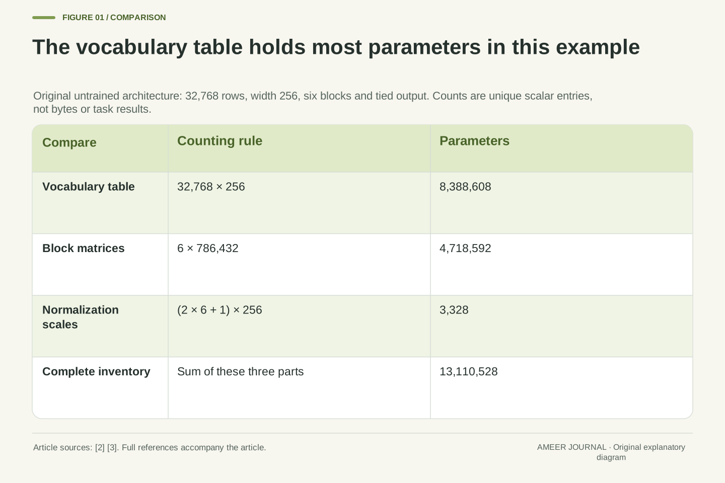
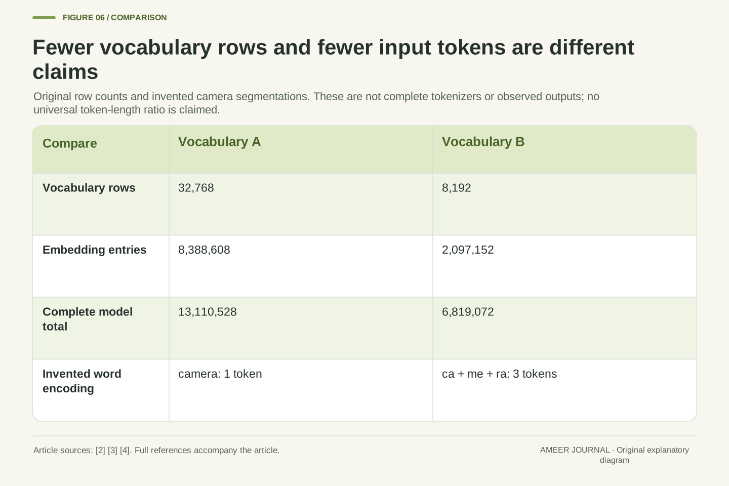
An embedding table has one row for each token identifier and one column for each vector component. PyTorch documents those two dimensions directly [2]. With 32,768 rows and 256 components in this example, the table contains 32,768 × 256 = 8,388,608 learned entries.
That number does not depend on how many different token identifiers appear in today’s prompt. A short input may read only a few rows, but our defined model still contains the complete table. Nor does a row necessarily stand for a whole written word. Token vocabularies can include smaller pieces and special symbols; the row count is the declared set of identifiers, not the number of words a reader recognizes [4].
The multiplication explains the structural cost. Increasing vocabulary adds more complete rows. Increasing width makes every existing row longer. In this particular design, the table will turn out to be larger than all six blocks’ matrix weights combined. That conclusion comes from the declared dimensions, without requiring any assumption about whether some token is frequent, useful or easy for the model to learn.
Let E have shape (V, d). Its unique scalar count is P_embedding=Vd=32,768×256=8,388,608. This follows from the documented lookup-table dimensions [2], with the values chosen for the exercise. V includes every declared vocabulary row; we do not silently exclude special identifiers or rows unused by a particular input.
A lookup retrieves selected rows but does not redefine the inventory as only those rows. Likewise, the output alias in the baseline does not add another Vd term. It reuses E as the output scoring weight, so the parameter object remains unique even though its role differs between row lookup and output projection.
The scaling is linear in V at fixed d and linear in d at fixed V. That differs from the quadratic d dependence of several block matrices below. Tokenization determines which discrete units receive identifiers, while the embedding width determines the number of values attached to each identifier [4]. The count does not establish linguistic coverage, semantic quality or the number of input characters that fit into a context. Those would require information beyond E’s shape.
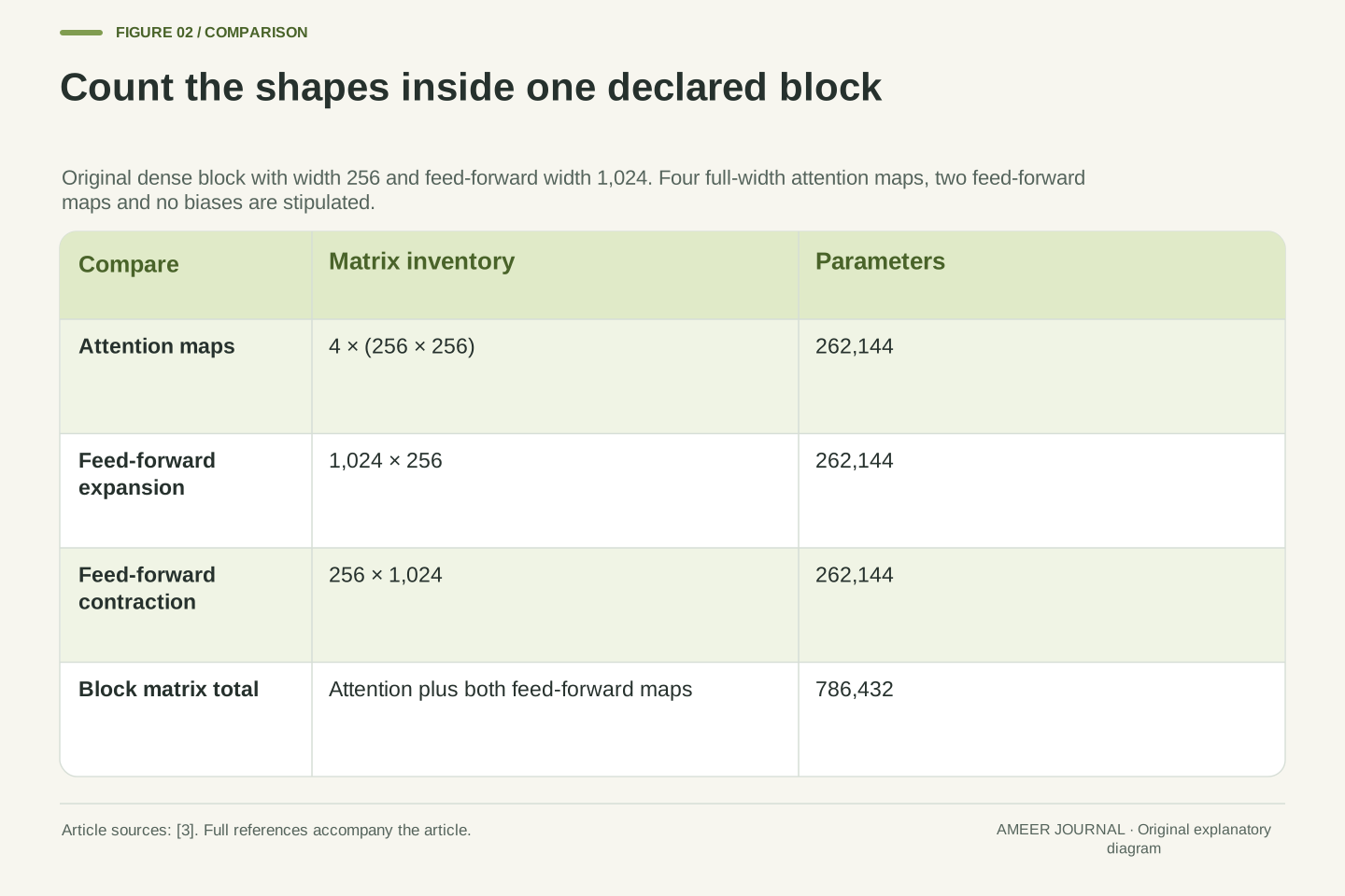
Count the matrices inside one block before multiplying by depth
Each square attention matrix has 256 × 256 = 65,536 entries. Four such matrices contribute 262,144 entries per block. The feed-forward expansion has 1,024 × 256 = 262,144 entries, and its contraction has the same count with the dimensions reversed. Those two together contribute 524,288.
Add the attention and feed-forward parts: 262,144 plus 524,288 gives 786,432 matrix entries in one block. Six distinct blocks therefore contain 4,718,592 matrix entries. That is already less than the vocabulary table’s 8,388,608. We still need to add the small normalization vectors before calling the inventory complete.
The method is ordinary matrix accounting. A dense map’s weight count comes from its input and output dimensions, with any bias counted separately [3]. Our design deliberately has no biases. The fixed activation adds no learned entries, but it still performs a computation. A component contributing zero parameters should not be mistaken for a component that does nothing. Parameter totals describe learned numbers, not every operation required to process a token.
For each full-width attention projection, the weight count is d²=65,536. The four projections contribute 4d²=262,144 per block. The two feed-forward maps contribute dm+md=2dm=524,288. Their shape convention is consistent with the documented dense-linear parameter layout [3]. Reversing the dimensions changes the map’s direction but not its element count.
Thus P_matrices_per_block=4d²+2dm. With m=4d, this becomes 12d²=786,432. Across L=6 independent blocks, P_block_matrices=12Ld²=4,718,592. Block independence matters: a design that reused one block’s parameter objects across repeated applications would need another counting rule.
No learned bias, gated third feed-forward matrix or reduced key/value projection is hidden in the formula. Fixed activations, attention normalization and other parameter-free operations add no learned scalars by declaration, although they still have execution costs. The four square projections are a specification of this exercise rather than a general inference from the word transformer. The remaining learned objects are the normalization scales, which must be added explicitly even though they are much smaller than the matrices.
The full count exposes when the vocabulary becomes dominant
Each block contains two vectors of 256 learned normalization scales, making 512 scales. Six blocks contribute 3,072, and the final normalization contributes another 256. The scale total is therefore 3,328. Adding all parts gives 8,388,608 vocabulary entries, 4,718,592 block-matrix entries and 3,328 scales: 13,110,528 unique parameters.
The vocabulary table accounts for about 63.98 percent of that total. This is an exact inventory with a rounded percentage, not a measured memory profile. The example also makes clear why depth is only one part of model size: more than half of the entries sit outside the repeated blocks.
There is a useful boundary in this design. At the same width and six-block depth, a vocabulary larger than 18,445 rows contains more entries than all the block matrices and normalization scales combined. Our 32,768-row vocabulary lies above that boundary. The threshold belongs to the declared architecture. It would change if the blocks gained extra matrices or if another learned component were added.
The learned normalization count is P_norm=2Ld+d=(2×6+1)×256=3,328. The complete tied-output inventory is P_total=Vd+L(4d²+2dm+2d)+d. Substituting m=4d gives P_total=Vd+12Ld²+2Ld+d=13,110,528.
The exact embedding fraction is 8,388,608/13,110,528, approximately 63.983754 percent. To determine when the table exceeds all other learned entries in this defined family, solve Vd>12Ld²+2Ld+d. Since d>0, this is equivalent to V>12Ld+2L+1. At L=6 and d=256, the right side is 18,445; the chosen V=32,768 satisfies the inequality.
This criterion makes the interaction between vocabulary, depth and width explicit. It is not an empirical law of model quality or a claim that embeddings always dominate small models. It holds only for the inventory just specified, including the tied output and absence of other learned tensors. We count the scale vectors even though omitting them would barely move the percentage, because an exact accounting example should preserve its declared boundary rather than quietly round away components.
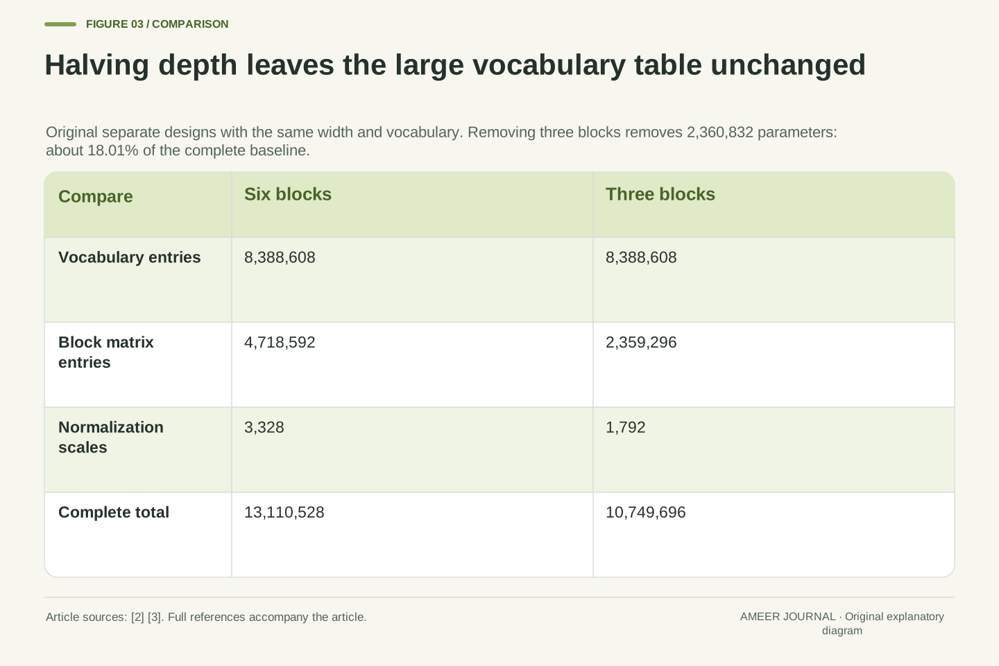
Half as many blocks removes only about eighteen percent here
Create a separate design with three blocks instead of six. Leave its 32,768-row vocabulary and 256-number width unchanged. The embedding table still contains 8,388,608 entries. Its block matrices now contain 2,359,296 entries, and its normalization scales total 1,792 because the final scale vector remains.
The new total is 10,749,696 parameters. Compared with the original 13,110,528, that removes 2,360,832 entries, or about 18.01 percent. The repeated block part has been halved, but the large shared vocabulary table has not changed. Counting only the blocks would therefore exaggerate the reduction in the whole model.
This is an architectural comparison, not an instruction to delete half the layers from a trained model. We have not established how any retained weights should change, whether the new network can perform the intended task or how long it takes to run. The result is narrower and useful: when most parameters sit outside the part being shortened, a large change to that part can produce a modest change to the total.
Set L=3 while retaining V=32,768, d=256, m=1,024 and tied output. Then P_block_matrices=3×786,432=2,359,296 and P_norm=(2×3+1)×256=1,792. The unchanged embedding term is 8,388,608, so P_total=10,749,696.
The difference is 13,110,528−10,749,696=2,360,832 parameters, approximately 18.007147 percent of the baseline. It equals the removed three blocks’ matrix entries plus their normalization scales: 3×(786,432+512). The final normalization vector and input/output table remain. The table’s share increases to approximately 78.04 percent even though its absolute count does not change.
No functional equivalence is implied. This comparison defines a different untrained architecture rather than a pruning or distillation procedure. It also does not establish an 18-percent latency change or any particular loss of capability. The mathematical lesson is the fixed term in the total: reducing L affects the repeated-block terms but leaves Vd present. That structure must be inspected before equating a layer-count ratio with a model-wide parameter ratio.
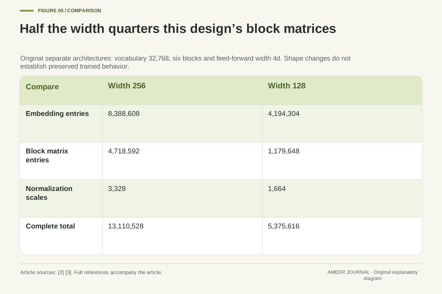
A narrower vector changes linear and quadratic terms differently
Keep six blocks and the same vocabulary, but reduce vector width from 256 to 128. Preserve the rule that feed-forward width is four times vector width, so it falls from 1,024 to 512. This is another separate architecture, with all its dimensions changed consistently.
The vocabulary table is halved to 4,194,304 entries. The block matrices shrink more: both dimensions of each relevant matrix are halved, so each matrix has one-quarter as many entries. Across six blocks they contain 1,179,648. Normalization scales are halved to 1,664. The complete total becomes 5,375,616 parameters, about 59.00 percent below the baseline.
This differs from simply making the model half as deep. Width changes the size of the vocabulary rows and several matrix dimensions at once. The arithmetic does not make width reduction the better choice for a task. It only shows why the same word smaller can describe different structural changes. Whether either design can learn or preserve the required behavior remains an evaluation question outside this untrained inventory.
Set d=128 and m=4d=512, retaining V=32,768 and L=6. The embedding term becomes Vd=4,194,304. Per-block attention contributes 4d²=65,536 and the feed-forward pair contributes 2dm=131,072, for 196,608 matrix entries per block. Six blocks therefore contribute 1,179,648.
The scale count is (2L+1)d=1,664, producing P_total=4,194,304+1,179,648+1,664=5,375,616. Relative to the baseline, this removes 7,734,912 parameters, approximately 58.997715 percent. The Vd and normalization terms scale linearly with d, while the block-matrix term scales quadratically because m remains proportional to d.
Those scaling relationships hold under the stated architecture and coordinated dimension change. They do not identify a universally best width/depth tradeoff. Changing d also changes the shapes that trained parameter arrays would need, so this is not an operation that preserves the baseline’s function by simply cropping columns. No training recipe or compensation procedure has been specified. The supported result is the new exact parameter inventory, with task quality and runtime behavior left unmeasured.
Fewer vocabulary rows leave the repeated block matrices alone
Return to the baseline width of 256 and six blocks, but choose only 8,192 vocabulary rows. That is one-quarter of the original row count. The embedding table now contains 8,192 × 256 = 2,097,152 entries. The blocks and normalization scales retain their original dimensions, totaling 4,721,920 entries together.
The new model total is 6,819,072 parameters. It is about 47.99 percent below the baseline, even though the vocabulary table itself became 75 percent smaller. The unchanged processing components explain the difference. This is the same accounting principle as the depth example, applied to another part of the model.
A vocabulary reduction also raises a question that the parameter count cannot answer: how will text be represented with the new set of token pieces? The tokenizer and its table must be designed together [4]. Our arithmetic specifies a possible row count. It does not specify a complete tokenizer, guarantee coverage of any language, or show that unused rows can be removed from a trained model without changing its behavior.
For the smaller-vocabulary variant, set V=8,192 with d=256, m=1,024, L=6 and tied output unchanged. Then P_embedding=2,097,152, while the nonembedding total stays 12Ld²+2Ld+d=4,721,920. Hence P_total=6,819,072.
The reduction is 6,291,456 entries, approximately 47.987816 percent of the baseline. Only Vd changes. A 75-percent reduction in V does not produce a 75-percent reduction in P_total because the remaining terms are fixed. If the output were independently parameterized, both vocabulary-sized tables would need to be included in a corresponding comparison; that is not this tied-output variant.
The count is a structural possibility, not a valid checkpoint migration. Vocabulary rows are associated with tokenizer identifiers and output symbols. The Hugging Face guide emphasizes the relationship between the tokenizer’s rules and the model’s training inputs [4]. Changing the inventory of symbols may require different segmentation, remapping and training decisions. Our hypothetical architecture has no trained state to preserve and supplies no evidence that any particular reduced vocabulary is sufficient for an application.
A smaller table can still produce a longer token sequence
Consider the word camera. In one invented vocabulary, it is represented by the single piece camera with identifier 3141. In another invented vocabulary, it is represented by the three pieces ca, me and ra, with identifiers 41, 72 and 105. Joining the pieces gives the same written word in both cases, but the sequence lengths are one and three.
These assignments illustrate the difference between vocabulary size and the number of tokens needed for a text. They are not outputs from a real tokenizer, and they do not prove that every smaller vocabulary makes every text longer. The documented idea of subword tokenization supplies the context: text can be composed from smaller known pieces [4]. Our particular pieces and identifiers are chosen only for the example.
The identifiers also belong to their own tables. Sending identifier 3141 to another model does not automatically mean camera there. The receiving table could assign that row another meaning. A parameter total therefore needs the associated tokenizer and mapping if someone is going to use the model. Knowing that two systems can represent the same characters does not make their token identifiers interchangeable.
Define two illustrative encodings of the literal string camera. Vocabulary A, associated with the 32,768-row example, uses pieces (camera) and IDs (3141). Vocabulary B, associated with the 8,192-row example, uses pieces (ca, me, ra) and IDs (41, 72, 105). All listed IDs lie within their declared ranges, and concatenating either piece sequence reproduces the same six-character string.
This is a finite encoding example, not a trained tokenizer or a complete vocabulary specification. Its lengths 1 and 3 show that table row count V and per-input sequence length are different variables. It does not establish a universal ordering between tokenizer vocabularies or a model-wide character-per-token ratio. The source’s subword discussion supports composing text from pieces, without supplying these invented outputs [4].
Identifier compatibility is equally separate from dimensions. A row index names a position within a particular mapping; equal numeric IDs across different vocabularies need not designate equal pieces. The source guide’s training/tokenization compatibility warning is relevant here [4]. Any real architecture comparison should retain the tokenizer identity and preprocessing rules alongside its parameter shapes. Those details are needed to interpret actual inputs even when the parameter-count arithmetic itself is correct.
Use the inventory to ask a better question about a small model
The five designs answer different accounting questions. Shortening the stack changes repeated blocks. Narrowing the vectors changes both table rows and matrix dimensions. Shrinking the vocabulary changes the table. Sharing the input and output weights avoids a second independent vocabulary-sized component. Each result can be explained from the part that changed.
None of those counts tells us which design gives the best answers. The examples have no learned values or task results. Even a complete parameter inventory cannot establish how much memory a particular runtime allocates, how smoothly output arrives or how well the model follows an application’s instructions. Those require the actual trained model and relevant measurements.
For a real comparison, retain the model’s identity, tensor shapes, sharing rules, tokenizer and task evidence. Google’s dated release describes its small model as intended for task-specific adaptation [1]; that intention should not replace checking the task you need. The useful outcome of the inventory is a precise explanation of what small means in the design. It prevents a depth label or one headline number from standing in for the whole architecture.
The derived comparisons are structural sensitivities within one explicitly defined family. Changing L affects repeated-block terms; changing d affects both linear and quadratic terms; changing V affects vocabulary terms; and untied output adds one independent Vd matrix. The original manifest lists every unique parameter object so each total can be reconstructed without relying on a model-size nickname.
These results provide no empirical ranking. There is no trained function, validation set, hardware configuration or serving trace in the exercise. Parameter totals also omit transient states and the numerical representation of each value. They should therefore remain architectural descriptors rather than proxies for deployment memory, inference latency, energy, language coverage or task correctness.
For an actual small language model, preserve exact version and configuration, all sharing relationships, tokenizer mapping and the task evaluation conditions needed to interpret its observed behavior. The dated Google release’s emphasis on task-specific adaptation provides context for asking about intended use [1], not evidence that our hypothetical designs work. An inspectable inventory establishes what was counted and which design decision changed it. Performance and capability claims require their own evidence on the resulting trained system.
Sources & further reading
Explore the references behind this guide. External pages may change after our review.
- Introducing Gemma 3 270M: The compact model for hyper-efficient AI
- Google Developers BlogGoogle · Accessed 7 Nov 2026
- Embedding — PyTorch 2.15 documentationPyTorch · Accessed 7 Nov 2026
- Linear — PyTorch 2.15 documentationPyTorch · Accessed 7 Nov 2026
- Summary of the tokenizers · Hugging FaceHugging Face · Accessed 7 Nov 2026
Article updated 7 Nov 2026.
Found something we should revisit?
Good explanations get better with thoughtful feedback.