What you’ll take away
- Query heads, stored KV heads and attention-head outputs are separate counts; grouped sharing does not remove query results.
- Two queries can combine the same stored values into (3, 2) and (1, 6); distinct queries can also agree under explicitly different conditions.
- Repeating histories that were already shared preserves the reference operands. Pooling independent histories does not generally preserve them.
- The declared 32-layer, batch-two, eight-KV-head cache contains 1 GiB of dense payload; total memory and runtime performance need separate evidence.
Eight questions can use two sets of stored information
A model description can list eight attention heads but only two key-value heads. That is not necessarily a missing part or a counting mistake. Grouped-query attention lets several query heads use the same stored keys and values [1]. A query supplies numbers used to decide how strongly to attend to each available position. Keys take part in that comparison, while values supply the numbers combined into the result. Sharing the keys and values does not require sharing the query that reads them.
Imagine eight readers using two notebooks. Readers zero through three use the first notebook, and readers four through seven use the second. The analogy concerns shared numerical information, not people inside a model. Each reader can look for something different. We will replace the analogy with exact invented vectors, including two different results obtained from the same stored values. Then we will separate this sharing arrangement from a very different operation: averaging information that was originally independent. No trained model or hardware experiment is involved.
Grouped-query attention separates the query-head count Hq from the key/value-head count Hkv. The original GQA paper assigns one key head and one value head to each group of query heads [1]. The distinction is architectural: fewer independently represented K/V histories need not mean fewer query results. PyTorch's pinned SDPA reference accordingly gives its query and output tensors a query-head axis, while K and V have their own head axis [2].
Our first construction has Hq=8, Hkv=2, one query position and two retained key positions. Query heads zero through three use KV group zero; heads four through seven use group one. Both retained positions are available to every illustrated query, dropout is zero, and query/key width is two. These are stipulated attention-level inputs, not embeddings extracted from a checkpoint. We examine grouping, output equality and logical cache payload without claiming equivalence of complete transformer models, observed allocation, inference speed or language quality.
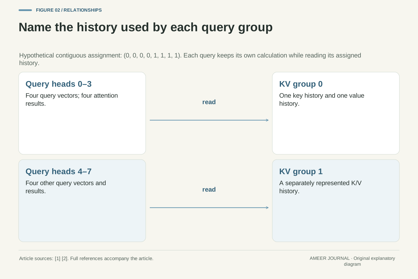
Read the query, stored-history and output counts separately
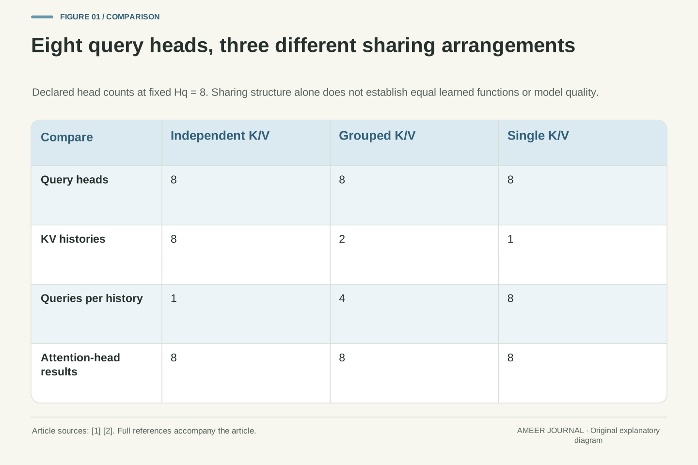
For the eight-query example, ordinary multi-head attention could keep eight separate key/value histories. Our grouped arrangement keeps two. A single shared key/value history gives the multi-query endpoint [1]. In all three descriptions, there are still eight query heads producing eight attention-head results. What changes is which histories they may use. Counting eight results does not tell you whether the storage contains eight different histories, two histories shared by groups, or one history shared by everyone.
The Transformers 4.49.0 Llama configuration documents separate num_attention_heads and num_key_value_heads fields, alongside the head dimension [3]. Those names help identify the intended roles when reading that version's configuration. They do not establish the settings of every model called Llama, or prove that an arbitrary file can be converted by changing a number. Start with the actual architecture description. A report that says only '32 heads' leaves a crucial question unanswered: does it mean queries, stored keys and values, or an output axis?
At fixed Hq=8, the comparison is Hkv=8 for independent multi-head K/V, Hkv=2 for the chosen grouping and Hkv=1 for the multi-query endpoint [1]. These counts describe sharing structure; they do not assert equal learned functions across the architectures. The attention output before any subsequent output projection still has Hq head results. In an axis convention using batch B, query length T and retained length S, we describe Q as (B,Hq,T,dk), K as (B,Hkv,S,dk), V as (B,Hkv,S,dv), and output as (B,Hq,T,dv) [2].
The pinned LlamaConfig documentation distinguishes num_attention_heads, num_key_value_heads and head_dim [3]. It also describes the MHA/MQA endpoints and grouped intermediate case. We use those explicit definitions rather than interpreting an ambiguous legacy num_heads cache-shape label as universally meaning Hq. Axis names and stored-head identity must come from the relevant contract. This article supplies no claim about the latest installed Transformers release, a particular downloaded checkpoint, or the physical arrangement of its cache buffers.
The same two values can give results of (3, 2) and (1, 6)
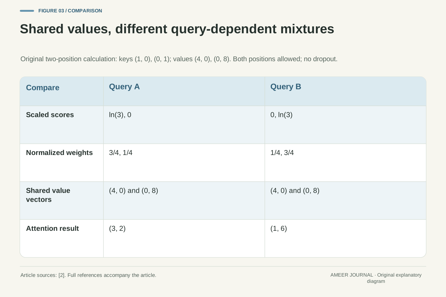
Give one shared history two key vectors, (1, 0) and (0, 1), and two corresponding value vectors, (4, 0) and (0, 8). Each pair of numbers is a vector with two coordinates. Choose query A so that, after scoring and the softmax conversion, its positive weighting strengths are in the ratio three to one. Its normalized weights are therefore three quarters and one quarter. Query B reverses that ratio. Different queries can produce those two weightings while using exactly the same keys; the Technical mode shows an explicit construction using the documented attention formula [2].
For query A, take three quarters of (4, 0) and one quarter of (0, 8). The result is (3, 2). For query B, take one quarter of the first value and three quarters of the second, giving (1, 6). Nothing in the shared value history changed between the two calculations. What changed was the query-dependent mixture. The results are attention vectors, not probabilities of two answers or measurements of intelligence. Their purpose is to make a precise point visible: sharing the ingredients does not force every query head to use the same proportions.
These ingredients also set a boundary. Giving more weight to (4, 0) raises the first coordinate while lowering the second. The two coordinates cannot vary independently in this particular mixture. Every result lies along the straight segment between the two stored value vectors; for finite scores, both weights are positive and the result lies between its endpoints. Shared values therefore permit different results within a defined set. They do not make every imaginable pair of numbers available to a query.
Let k0=(1,0), k1=(0,1), v0=(4,0), v1=(0,8), and dk=2. Using the default scale 1/sqrt(2), choose qA=(sqrt(2) ln(3),0) and qB=(0,sqrt(2) ln(3)). Their scaled score pairs are respectively (ln(3),0) and (0,ln(3)). Softmax therefore yields (3/4,1/4) and (1/4,3/4). This is an original exact construction from the scaled-score, softmax and value-product relationship documented by SDPA [2], with both positions allowed and no dropout.
The weighted outputs are oA=(3/4)v0+(1/4)v1=(3,2) and oB=(1/4)v0+(3/4)v1=(1,6). Both queries may belong to the same KV group; their scores and weights remain query dependent. The computation does not create a separate stored history for each result. Nor does it identify a full model's final hidden state: learned projections and later processing are outside this fixture. Exact fractions establish the teaching outputs; a separate floating-point calculation checks the logarithmic query construction within its stated numerical tolerance.
Writing the first weight as w gives output (x,y)=(4w,8(1-w)), hence x/4+y/8=1. With both scores finite and both positions allowed, 0<w<1, so the available outputs lie in the open segment between the two values. The endpoints are limiting cases as the score difference diverges, not exact finite-logit outputs under these assumptions. This original geometric observation separates output diversity from independent output coordinates. It applies before output projections and does not assert a corresponding constraint on the complete network's final representation.
Different queries are allowed to agree, too
The example proves that shared histories can produce different results. It does not prove that every pair of query heads must differ. Keep the same keys and values, but use a query that gives the two positions equal scores. Equal scores receive equal weights, so the result is half of (4, 0) plus half of (0, 8), or (2, 4). Several different queries can produce that same balance. Sharing neither demands identical outputs nor guarantees diversity; the actual numerical relationship decides.
There is a second way agreement can occur. Imagine replacing both stored values with the identical vector (5, 7). Three-quarter versus one-quarter weighting now makes no difference: every normalized mixture of those two identical values is still (5, 7). This deliberately simple boundary helps interpret a test. If every value in a test is identical, a wrong weighting may remain invisible in the output. To explore whether queries use a shared history differently, choose values that can distinguish the possibilities instead of treating one matching result as proof that all intermediate relationships match.
For the same identity-like keys, qC=(0,0) gives logits (0,0), while qD=(sqrt(2) ln(3),sqrt(2) ln(3)) gives (ln(3),ln(3)). The queries differ, but both weight vectors are (1/2,1/2) and both outputs are (2,4). Adding the same constant c to every score leaves softmax unchanged because its common exp(c) factor cancels between numerator and denominator. This is an algebraic consequence of the normalization in the cited formulation [2], not a measured behavior of a trained head.
Output equality is weaker still than weight equality when the values conceal the distinction. With v0=v1=(5,7), both (3/4,1/4) and (1/4,3/4) produce (5,7). More generally, any normalized weighting of identical vectors returns that vector. Thus a grouping diagnostic should compare the assigned K/V groups and intermediate reference weights as well as outputs. Our two-coordinate examples deliberately include distinguishable values for the unequal-output case, then a degenerate case showing why output agreement alone cannot establish complete semantic agreement.
For two normalized weight rows with first components a and b, subtracting their outputs gives (a-b)(v0-v1). When v0 differs from v1, equality of these two outputs requires a=b; when the values coincide, the difference vanishes for any a and b. For a general value matrix V, the corresponding condition is that the difference of the weight rows multiplied by V equals zero. This is an algebraic equality criterion for the declared weighted sum, not evidence that a trained model has or lacks useful differences between its heads.
The order of the groups is part of the computation
With eight queries and two groups, our contiguous assignment is (0, 0, 0, 0, 1, 1, 1, 1). Each number says which history that query head reads. Alternating the two histories would instead give (0, 1, 0, 1, 0, 1, 0, 1). Both assignments have eight entries and use each history four times. Their totals look equally reasonable, but several query heads now read a different history. A matching tensor size cannot reveal which assignment was intended.
To expose the difference, make all queries zero so each history's two positions receive equal weights. Keep group zero's values (4, 0) and (0, 8), whose mean is (2, 4). Give group one the values (10, 2) and (-2, 6), whose mean is (4, 4). Query head one returns (2, 4) under our contiguous map and (4, 4) under the alternating map. The calculation isolates the group assignment: neither the values nor the query changed. PyTorch's illustrative repeat_interleave formulation corresponds to consecutive repetitions [2]; another layout needs its own explicitly correct mapping.
For contiguous equal-size groups, let r=Hq/Hkv and g(h)=floor(h/r). At Hq=8,Hkv=2, r=4 yields g=(0,0,0,0,1,1,1,1). The pinned SDPA formulation repeats each K/V head consecutively, and its native constraints require query-head divisibility by KV-head count and equal key/value head counts [2]. Those constraints belong to that documented interface. They are not permission to substitute a different tiling order merely because the resulting head-axis length is Hq.
Using zero queries and two allowed positions, group-zero values average to (2,4), while group-one values (10,2),(-2,6) average to (4,4). Replacing g(h) with h modulo 2 changes outputs for heads 1,3,4,6 in the eight-head fixture. We calculate those four differences explicitly. A permutation can be harmless if all affected query, group and output identities are transformed consistently; this counterexample instead changes only the association. Its lesson concerns semantic indexing, not a claim that a particular framework makes this error.
Repeating shared values is different from merging independent ones
Suppose we already have the two shared histories. For a reference calculation, we could make four identical copies of each and give one copy to every query in its group. Each query would still receive the same numbers, so the mathematical result would be unchanged. This is a way to explain a sharing operation. It does not mean that every efficient implementation actually makes those copies in memory. The documentation's equivalent formulation describes a relationship, while an implementation's storage choices require separate evidence [2].
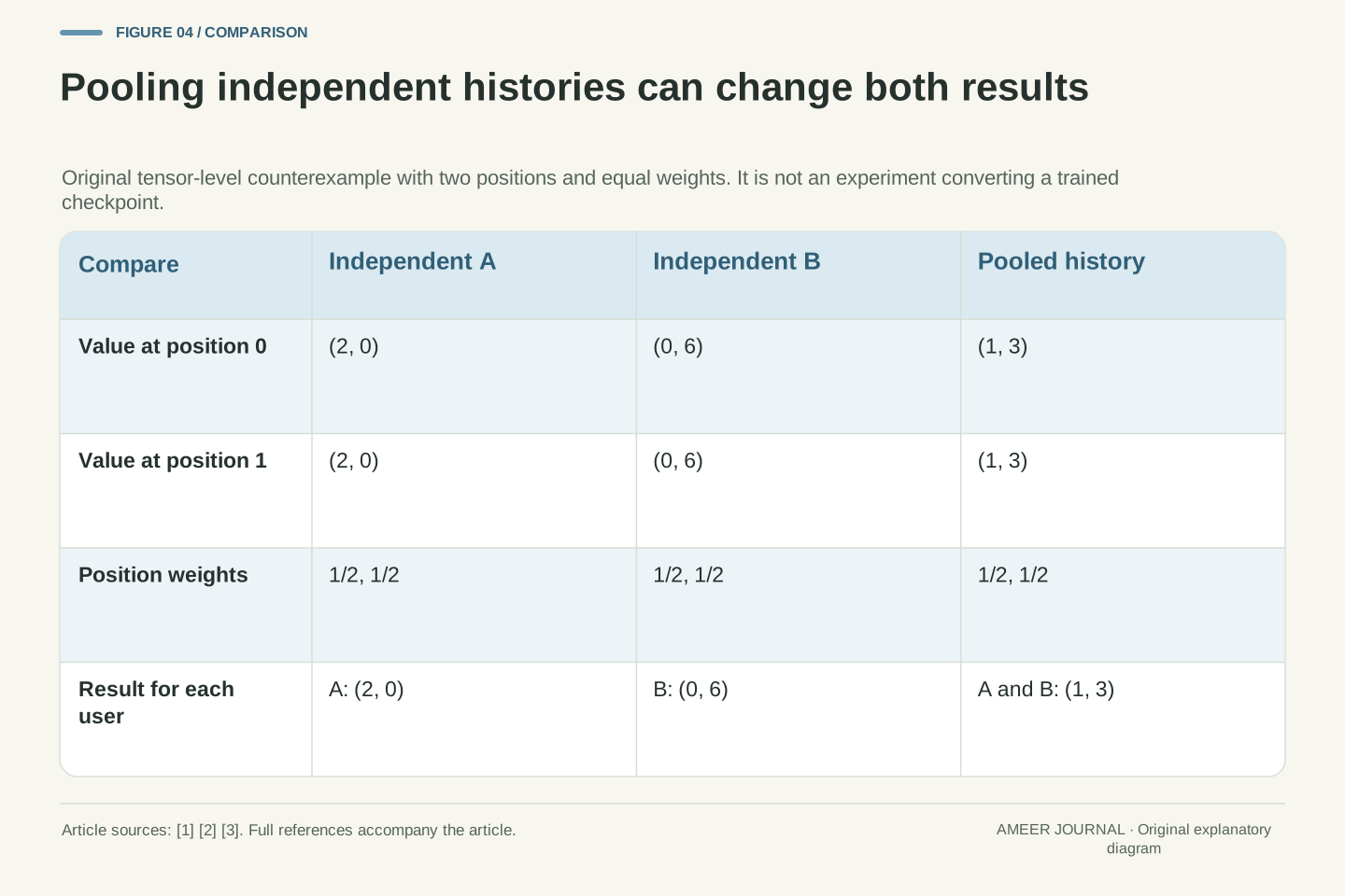
Now start from genuinely independent histories. Let head A have (2, 0) at both positions, and head B have (0, 6) at both positions. Use zero scores, so each head averages its own values. Their results are (2, 0) and (0, 6). Averaging the histories together gives (1, 3) at both positions; both results become (1, 3). This tensor-level counterexample shows why merging arbitrary histories is not automatically lossless. The original GQA work describes checkpoint conversion followed by additional training [1]. That is a different task from repeating information that was already shared.
Given a valid grouping g, define expanded K'_h=K_g(h) and V'_h=V_g(h). Holding each Q_h, mask and scale fixed, independent-head attention over these repeated tensors equals grouped attention in exact arithmetic: every head receives identical operands. PyTorch's equivalent formulation expresses this repetition [2]. The identity concerns already shared inputs. It does not prove identical allocator behavior or bitwise equality across kernels using different finite-precision evaluation orders, both of which lie beyond this reference construction.
For the converse, take two independent heads with zero scores and constant values A:(2,0),(2,0) and B:(0,6),(0,6). Their outputs are (2,0) and (0,6). Positionwise mean pooling makes both value positions (1,3), hence both shared outputs (1,3). This is a constructed tensor-level counterexample, not a conversion experiment on trained weights. The GQA paper and pinned Llama configuration discuss mean pooling in checkpoint conversion [1][3]; the paper also describes adaptation through further training. Neither description establishes universal exact preservation of an arbitrary original MHA function.
Count stored heads when counting stored bytes
The group map tells us why the cache estimate uses stored key-value heads rather than the number of queries that read them. In a simple dense representation, every retained position has one key vector and one value vector per KV head. If four queries use the same stored history, counting that history four times would describe a physically expanded reference, not the compact representation we set out to count. The declared storage boundary must come before the multiplication.
For one layer, multiply the number of independent sequences by retained positions, then by KV heads. Multiply again by the total number of coordinates in a key plus a value, and by the bytes used for each coordinate. Sum across layers. These are our element-counting steps for the explicit tensor shapes [2]. They assume every counted layer has the stated dimensions and storage precision. We are counting dense K/V payload alone: no claim is made that the resulting number includes model weights, spare allocation, metadata or temporary computation.
For dense unexpanded K shaped (B,Hkv,S,dk) and V shaped (B,Hkv,S,dv), at b bytes per element for both tensors, one layer's payload is B S Hkv (dk+dv) b bytes. For L homogeneous layers it is L B S Hkv (dk+dv) b. When dk=dv=d, this becomes 2 L B S Hkv d b. The derivation counts the elements of the declared K/V axes [2]; Hq is absent because this representation stores each grouped history once.
The expression is conditional on the representation. Layer-specific dimensions require summing the corresponding layer terms. Different K/V element sizes require separate byte factors. Expanded copies, padding or additional representation data require additional accounting. We do not infer a device allocation trace from an architecture field or from the reference repetition code. This same separation also explains why a query-output tensor with Hq heads does not invalidate a cache tensor with only Hkv heads: they contain different objects and belong to different parts of the computation.
As a separate architectural thought experiment, increasing Hq from 32 to 64 while holding Hkv, retained positions, K/V widths and precision fixed leaves this compact K/V payload unchanged. The query and attention-output head axes grow, and the number of queries per group changes. Those objects and any extra computational work are outside the stored-payload expression. This is another reason to name the counted tensor instead of calling every head-dependent quantity 'cache memory'.
A complete ledger gives 1 GiB for the declared grouped cache
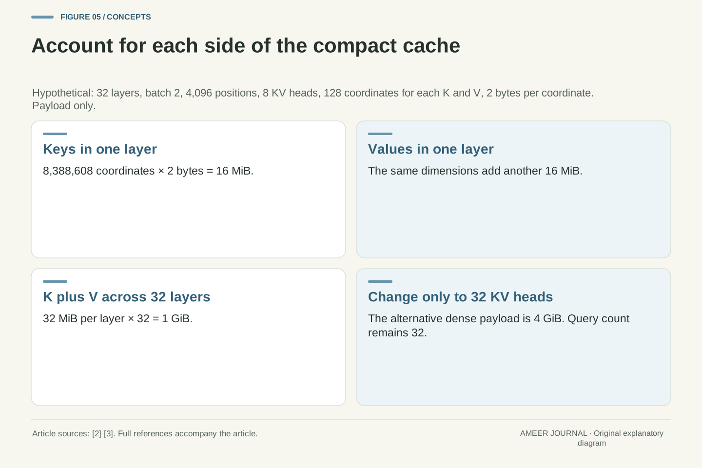
Use a larger invented configuration for a storage example: 32 layers, two independent sequences, 4,096 retained positions per sequence, 32 query heads and eight KV heads. Each key and each value has 128 coordinates, stored at two bytes per coordinate. The query count helps describe the sharing ratio, but eight is the head count used in the cache multiplication. These numbers are chosen for clear arithmetic; they are not the specification of a real product.
One layer's keys contain 2 × 4,096 × 8 × 128 = 8,388,608 coordinates. At two bytes each, that is 16 MiB. Values take another 16 MiB, so the layer needs 32 MiB of dense K/V payload. Across 32 layers, the total is 1 GiB, or 1,073,741,824 bytes. Here MiB means 1,048,576 bytes and GiB means 1,073,741,824 bytes. Keeping every other assumption fixed but using 32 independent KV heads would give 4 GiB. The fourfold comparison concerns these stored tensors, not the entire model or its execution time.
Set L=32, B=2, S=4096, Hq=32, Hkv=8, dk=dv=128 and b=2 bytes. Keys per layer contain 2·4096·8·128=8,388,608 elements and 16,777,216 bytes. Values have the same count. Combined per-layer payload is 33,554,432 bytes=32 MiB; multiplying by 32 layers gives 1,073,741,824 bytes=1 GiB. Binary units are defined by MiB=2^20 bytes and GiB=2^30 bytes.
At otherwise identical dimensions, Hkv=32 gives 4 GiB and Hkv=1 gives 128 MiB. These are alternative stipulated storage architectures, not claims that an existing checkpoint can be changed between them without adaptation. The same 1 GiB payload budget would contain S=1024 positions per sequence at Hkv=32, versus S=4096 at Hkv=8, under these homogeneous assumptions. That inverse calculation establishes an element budget only. It does not extend a trained context window, reserve room for weights, establish supported allocation, or guarantee that either full workload fits on a particular device.
A sharing ratio does not settle the workload or runtime
The fourfold saving above holds because we changed one factor: stored heads. If we keep eight KV heads but increase the batch from two independent sequences to eight, the cache returns to 4 GiB. The architecture still shares four query heads per KV group. The workload simply asks it to retain four times as many equally long sequences. A report can therefore truthfully describe head sharing while showing no reduction against a different, smaller batch. Compare the declared factors before judging the result.
Likewise, a 1 GiB K/V payload is not a claim of 1 GiB total memory. Other resident data and temporary work are outside that count. The attention documentation describes implementation selection and numerical differences between kernels [2], so the illustrative repeat operation cannot establish an actual allocation or timing result. A useful performance report needs observations from the chosen model, software, workload and hardware. Our calculation answers which entries are counted. It does not predict how quickly those entries are read or whether the resulting model answers a question well.
With other factors equal, the dense grouped-to-independent payload ratio is Hkv/Hq, here 8/32=1/4. Across different workloads the ratio instead includes the other changed factors. In our explicit comparison, (B,Hkv)=(8,8) and (2,32) have the same product 64 and therefore the same 4 GiB payload at the fixed L,S,d,b. This algebra prevents attributing a cross-workload total solely to architecture. It does not imply that those batches have equal latency, throughput or scheduling behavior.
Logical storage, allocator capacity and measured peak memory are different quantities. The first can be derived from a stated representation; the latter two need implementation evidence. The pinned SDPA reference permits backend-dependent computation and warns about numerical differences [2]. Its equivalent repeat code does not prove persistent replicated cache storage in every backend. Similarly, the historical GQA paper's empirical trade-offs have their own model and evaluation scope [1]. We make no transfer of those results to the invented eight-query fixture or the 32-layer byte ledger.
Use a reference that checks sharing, outputs and the counting boundary
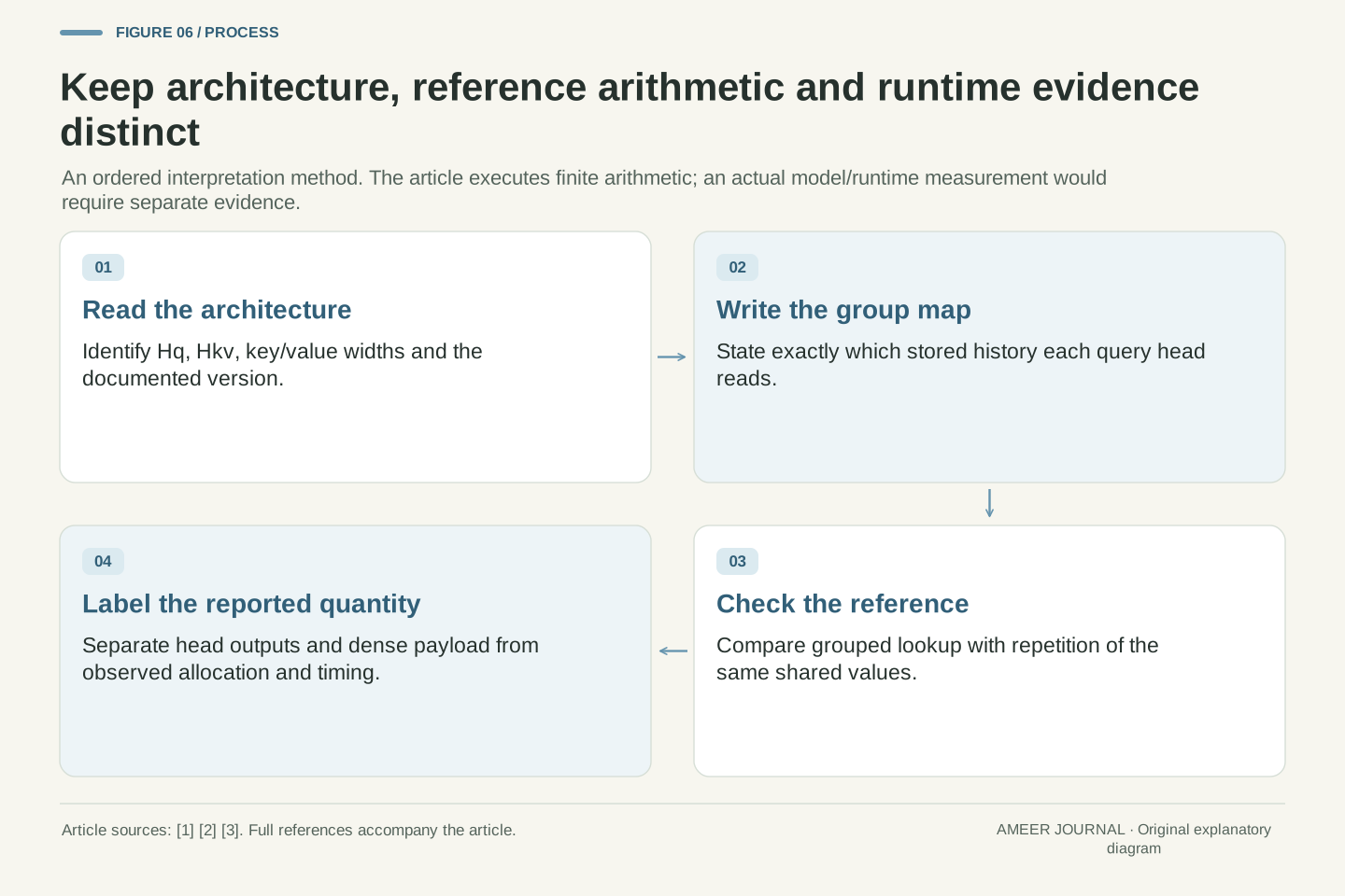
A useful record starts with the separate query and KV head counts, then names the group used by each query. Give the groups distinguishable values so that swapping them can be detected. Next compare a grouped calculation with a reference that repeats only the histories already intended to be shared. Our own bounded arithmetic checks cover 210 such constructed cases and preserve the eight-query example's exact output vectors. They check the stated mathematics; they do not certify a framework, checkpoint or device.
Finally, label the number you are reporting. An output vector answers what a query retrieved from the available values. A payload total answers how many bytes the defined stored tensors contain. A runtime measurement would answer another question and would need an actual execution record. Read the architecture fields in their documented version [3], preserve the grouping relation [2], and keep those conclusions separate. Eight query heads with two KV histories is then a precise, understandable arrangement: several distinct calculations can read shared numerical material without requiring a separate stored copy for every result.
The retained reference enumerates Hq from 1 through 12, every positive divisor Hkv of Hq, and six rational-weight fixtures for each valid pair: 210 constructed cases. It compares direct group lookup with consecutive expansion of the same values, using exact fractions for the weighted outputs. Separate checks retain the logarithmic score construction, common-score-shift equality, identical-value degeneracy, alternating-map discrepancy, pooling counterexample and byte ledger. No PyTorch operator, model inference, checkpoint transformation or GPU-memory measurement is executed.
For a real implementation, record Q/K/V axis meanings, the query-to-group association, supported head constraints, masks, scale, precision and the actual output boundary. Then report the compact cache representation separately from temporary or reserved allocations. The pinned configuration and SDPA references establish named contracts [2][3], while our arithmetic supplies small cases that explain the intended relationships. The central distinction is preserved throughout: repetition of already shared histories can preserve an attention calculation, whereas replacing independent histories with pooled ones changes its operands and needs its own justification.
Sources & further reading
Explore the references behind this guide. External pages may change after our review.
- GQA: Training Generalized Multi-Query Transformer Models from Multi-Head CheckpointsAinslie et al. / Google Research / arXiv · Accessed 7 Nov 2026
- torch.nn.functional.scaled_dot_product_attention — PyTorch 2.15 documentationPyTorch contributors · Accessed 7 Nov 2026
- LLaMA · Hugging FaceHugging Face · Accessed 7 Nov 2026
Article updated 7 Nov 2026.
Found something we should revisit?
Good explanations get better with thoughtful feedback.