An assistant can start answering quickly and then stop moving for an uncomfortable stretch. Another can take longer to begin, but deliver the rest in a steady rhythm. If both finish at the same moment, a single total-time number hides much of what the reader experienced. A first-response number hides a different part of the story.

We will follow five invented requests using exact arrival times for their streamed output. The first three let us compare response speed and averaging. A fourth delivers several tokens in one event. The fifth produces only one token. Every timestamp is constructed for this explanation; no model, server or internet connection was benchmarked.

The distinction has a practical counterpart in vLLM’s version 0.31.0 documentation, which separates first output, gaps between outputs and average time per later output token [1]. These measurements answer different questions. Before deciding that one assistant is faster, identify which part of the wait matters and what was actually timed. The same trace can support several correct numbers without those numbers being interchangeable.

Streaming latency is a collection of observables with different boundaries and aggregation units. Time to first token, inter-output gaps, completion latency and per-request amortized time per output token need not rank traces identically. A comparison becomes ambiguous when its metric label substitutes for a specified event definition.

The following fixtures declare every client-observed content event. A, B and C contain one output token per event; D contains a multi-token event; E contains only one output token. Each request has its own send-time origin at zero milliseconds. These origins do not establish a common workload window or concurrency schedule. All requests succeed, and their completion boundaries coincide with their final content events by construction.

We apply the definitions documented in vLLM v0.31.0 and compare one differently normalized definition from NVIDIA’s GenAI-Perf README [1][3]. No implementation was executed. The purpose is to derive exact consequences of declared traces, including event weighting and undefined denominators. The fixtures exclude empty role frames, tool calls, hidden output and retry traffic; they therefore cannot establish how an arbitrary API or user interface handles those cases.

Start our timer when the client sends a request. Record when that same client receives each content event and when the request finishes. The first-token time is the first event’s arrival minus the send time. Total response time runs from sending to completion. A gap is the difference between two consecutive event arrivals.

These boundaries leave some things unknown. The records do not say when a person clicked a button, when text first appeared on a screen, or when the server began computing. A browser could receive content before showing it. A client could also hold work before sending it. Those would require additional timestamps, rather than being silently included in the numbers we already have.

The vLLM benchmark documentation explicitly distinguishes waiting for a client concurrency limit from its ordinary request timing [1]. That distinction is useful even without using the tool: name the starting event. Our examples begin at sending, use one consistent timing basis within each request, and contain no recorded wait before sending. They cannot tell us whether such a wait occurred elsewhere.

For request r, let s_r be its client send timestamp, a_r,j its content-event arrival timestamps, f_r its completion timestamp and N_r its declared output-token count. Define TTFT_r=a_r,1−s_r, L_r=f_r−s_r and g_r,j=a_r,j−a_r,j−1 for j≥2. In these fixtures, f_r equals the last content arrival; that equality is a modeling premise, not a general protocol rule.

Use compatible interval timestamps. The vLLM metrics discussion recommends monotonic timing to avoid changes in the wall clock [2]. Our calculation assumes such a stable client timing basis and does not subtract unvalidated timestamps from unrelated clock domains. The documents’ implementation details about particular process clocks should not be treated as universal operating-system behavior.

The pinned benchmark guide separately exposes client-concurrency waiting and describes a schedule-relative completion metric under specified request-rate settings [1]. We have no scheduled-arrival or browser-paint events. Consequently, our L is neither a click-to-paint duration nor a full scheduled-workflow duration. It is also not a decomposition into network, server queue and computation time; those components remain unobserved by this client-only fixture.

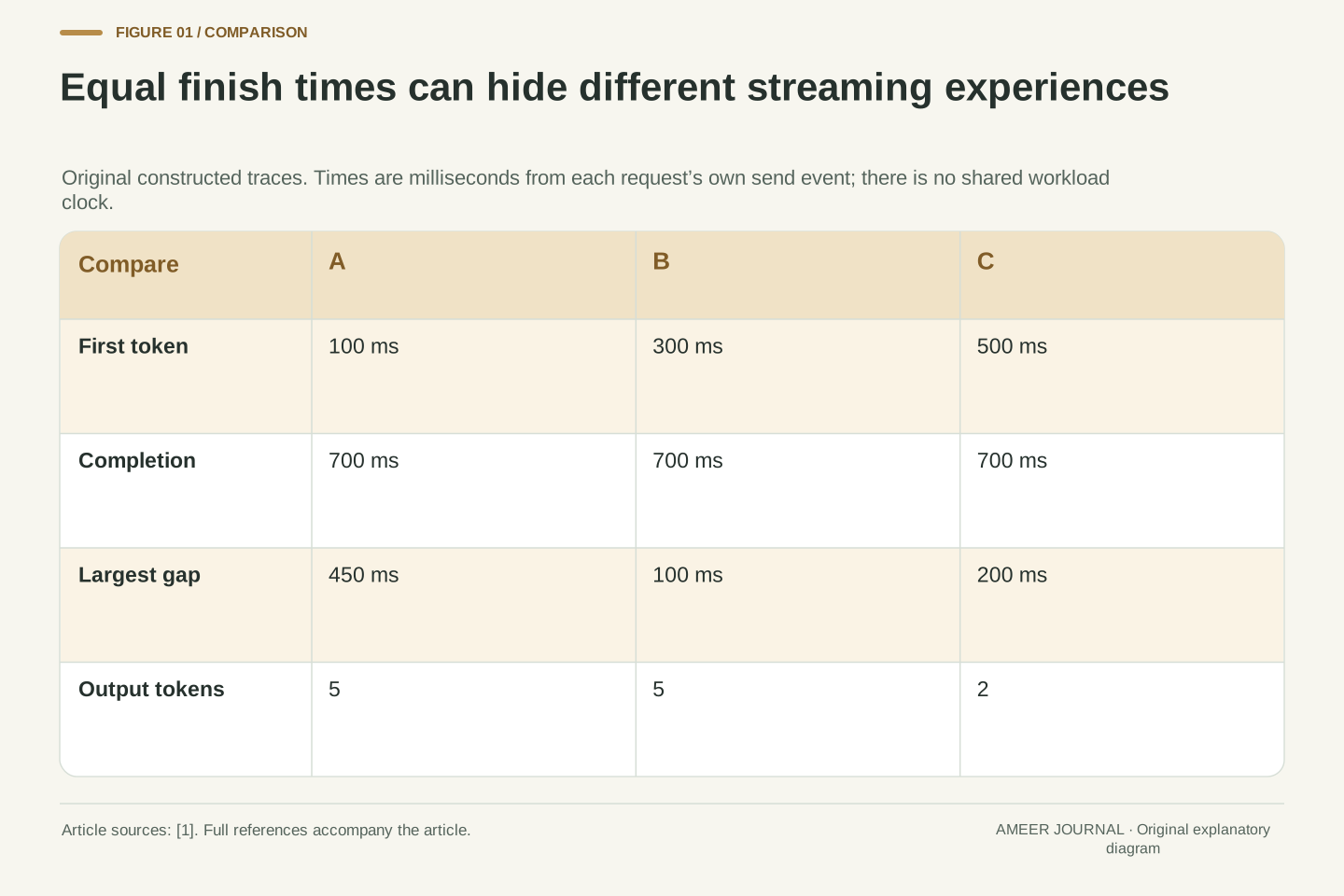
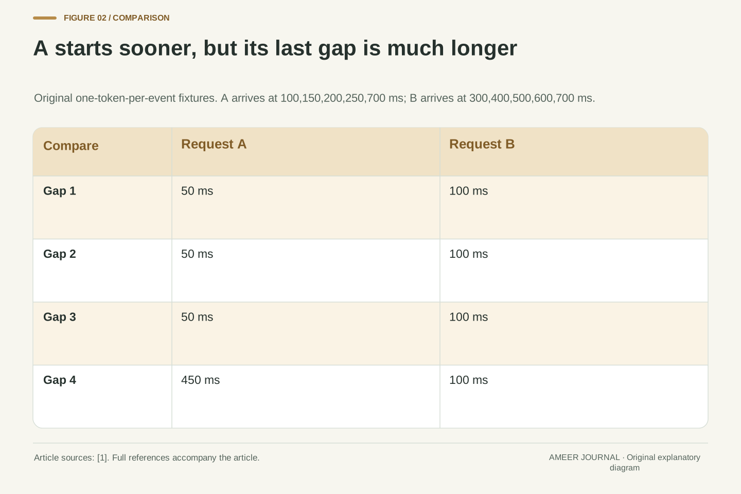
Request A delivers its five tokens at 100, 150, 200, 250 and 700 milliseconds. Request B delivers five tokens at 300, 400, 500, 600 and 700 milliseconds. Each list is measured from that request’s own send time. Both requests therefore finish after 700 milliseconds and produce the same declared number of tokens.

A starts 200 milliseconds sooner. Its first three gaps are only 50 milliseconds each, but its final gap is 450 milliseconds. B begins later and then has four equal gaps of 100 milliseconds. The smaller first-response time belongs to A; the smaller largest pause belongs to B. Neither distinction changes the equal finishing time.

Imagine a reader seeing each event immediately. A would appear responsive at first and then pause, while B would begin later and continue steadily. That is an interpretation of the arrival pattern, not a measured user study. The actual screen experience could differ if the interface groups or delays updates. The records establish arrival timing; they do not reveal why A’s long gap happened.

Take A arrivals as (100,150,200,250,700) ms and B arrivals as (300,400,500,600,700) ms, with s=0 and N=5 in each case. Their first-arrival times are TTFT_A=100 ms and TTFT_B=300 ms. Their completion latencies are both L=700 ms.

The corresponding gap vectors are g_A=(50,50,50,450) ms and g_B=(100,100,100,100) ms. Therefore max(g_A)=450 ms and max(g_B)=100 ms. A improves the declared first-arrival measure relative to B, while B improves the declared maximum inter-output gap. Equal N and L are insufficient to reconstruct either gap vector.

All of these are exact properties of the constructed client traces. There is no inferred generation schedule inside the server. In particular, the 450 ms arrival gap does not identify a 450 ms model execution, network stall or queue event. Nor is the maximum of four gaps an estimated high percentile of a production population. Retaining the individual arrivals preserves information that a completion total and output count alone would discard.

For requests that produce more than one token, the documented per-request calculation subtracts first-token time from total time, then divides by the number of later tokens [1]. A has 600 milliseconds after its first arrival and four later tokens. Its result is 150 milliseconds per later token. B has 400 milliseconds after its first arrival and the same four later tokens, giving 100 milliseconds.

A’s average of 150 does not mean that each pause lasted 150. Its actual pauses were 50, 50, 50 and 450. The average combines them and loses their order. B’s average happens to equal every gap because we deliberately made its spacing uniform. An average alone cannot tell us which of these patterns occurred.

Add request C, which delivers two tokens at 500 and 700 milliseconds. It starts later than A or B, finishes after the same 700 milliseconds, and has one later-token gap of 200 milliseconds. We now have three per-request averages: 150, 100 and 200. The next question is how to combine them without changing what each observation represents.

For N_r>1, use TPOT_r=(L_r−TTFT_r)/(N_r−1), following the pinned benchmark definition [1]. Because every event in A, B and C contains one token and completion equals the last event, this is also the arithmetic mean of that request’s N_r−1 observed gaps. Those premises are necessary for the equivalence used here.

A gives (700−100)/4=150 ms/token. B gives (700−300)/4=100 ms/token. Define C by arrivals (500,700) ms and N_C=2; its value is (700−500)/1=200 ms/token. The numerator excludes time before the first observed token. Accordingly, the reciprocal of this average, with the appropriate unit conversion, would describe an amortized post-first-token rate, not whole-request completion speed.

TPOT_A summarizes an unequal gap sequence and does not certify uniform delivery. No token in A is observed after a 150 ms interval. The value arises from averaging three 50 ms intervals with one 450 ms interval. Keeping the raw gaps alongside the per-request mean allows a reader to distinguish regular spacing from a delayed final event without inferring any hidden implementation cause.

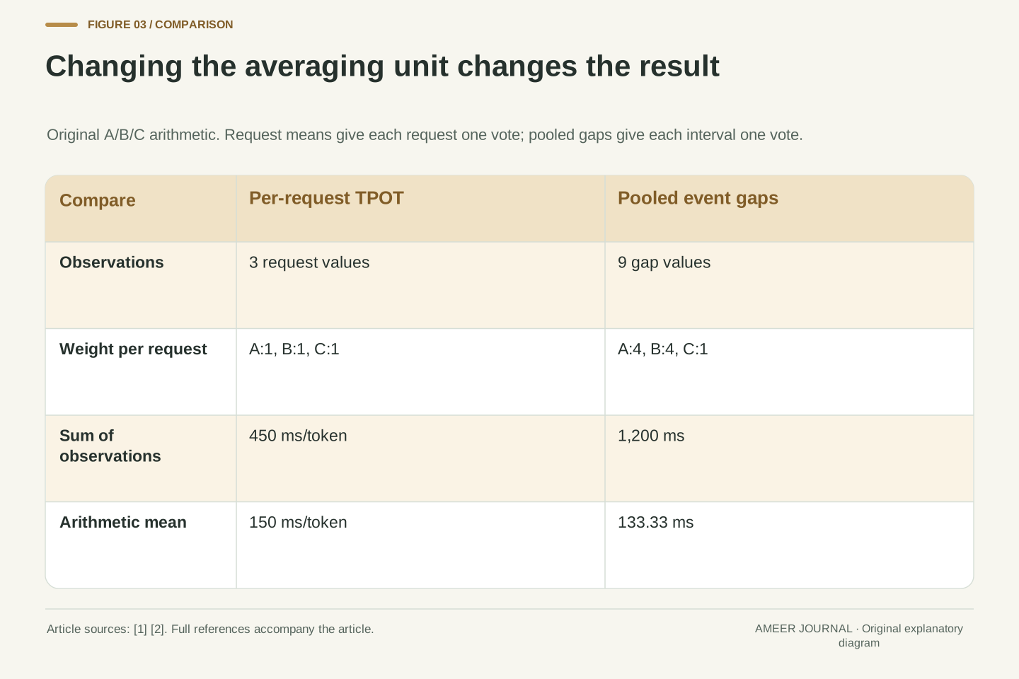
Give each of A, B and C one equal vote. Their average time-per-token values are 150, 100 and 200 milliseconds. Adding those three numbers and dividing by three gives 150 milliseconds. That answers a question about the average of the three request-level values.

Now combine every observed gap. A contributes four gaps totaling 600 milliseconds. B contributes four totaling 400. C contributes one totaling 200. There are nine gaps with a combined duration of 1,200 milliseconds, so the average gap is about 133.33 milliseconds. C has one vote in this calculation, while A and B each have four.

Neither result is an arithmetic mistake. They count observations differently. The vLLM documents distinguish statistics over streamed-output gaps from statistics over one calculated value per request [1][2]. A report that says only average token time leaves that choice unclear. Preserve the unit being averaged: a request or a gap. Our three-request set is deliberately small, so neither result estimates a wider population or proves how a service will behave under load.

The equally weighted request mean is mean(TPOT)=(150+100+200)/3=150 ms/token. Pooling the gap samples instead gives mean(g)=(600+400+200)/(4+4+1)=1,200/9=400/3 ms, approximately 133.333 ms. There are nine observations in the second calculation and three in the first.

For these one-token-per-event fixtures, the pooled mean is the weighted request mean with weights N_r−1: sum_r[(N_r−1)TPOT_r]/sum_r(N_r−1). It therefore assigns weights four, four and one. The unweighted request mean assigns weight one to every request. The vLLM metrics discussion explicitly identifies differing aggregation weights as a reason its inter-output and request-level summaries can diverge [2].

The formulas coincide under some special configurations, including equal numbers of intervals per request, but that condition is absent here. Neither aggregation is universally preferable. They estimate different descriptive quantities for the declared dataset. A monitoring or benchmark comparison should state the sample unit and inclusion rule before interpreting a difference as a change in model performance. No inference about unseen requests follows from this finite enumeration.

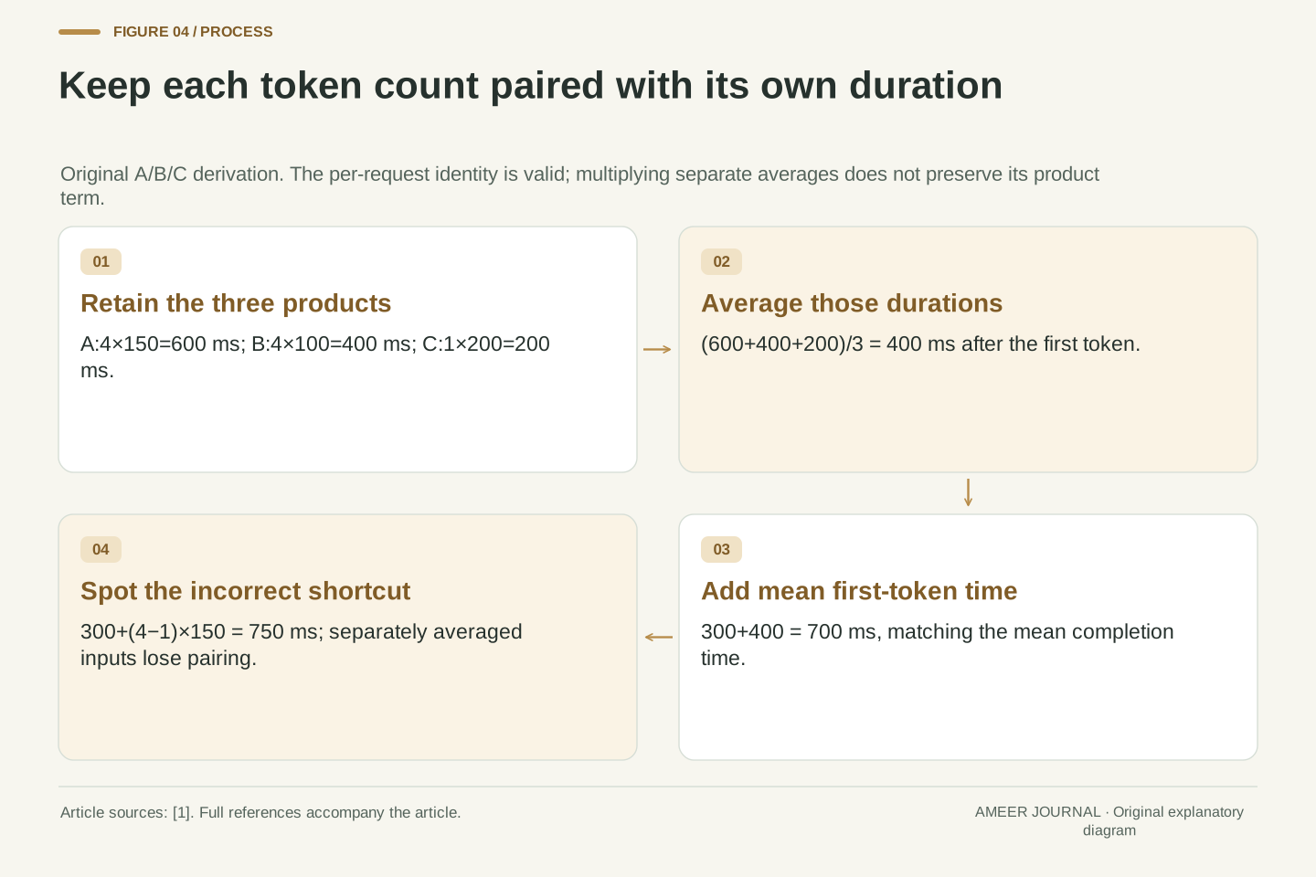
For each of our first three requests, total time equals first-token time plus the time after the first token. That last part also equals the number of later tokens multiplied by the request’s average time per later token. The equation works exactly for A, B and C.

It is tempting to insert three separate averages into it. Mean first-token time is 300 milliseconds, mean token count is four, and mean per-request token time is 150 milliseconds. The calculation becomes 300 plus three times 150, or 750 milliseconds. But every request actually finishes after 700 milliseconds, so their average completion time must also be 700.

The mistake is separating quantities that belong to the same request. A and B each contribute four later tokens; C contributes one. Instead, calculate the after-first duration for each request: 600, 400 and 200 milliseconds. Their average is 400. Add the mean first-token time of 300, and the correct mean completion time is 700. Keep the paired counts and durations together before averaging.

The identity L_r=TTFT_r+(N_r−1)TPOT_r holds for each r in {A,B,C} under the stated definition. Averaging preserves the identity as mean(L)=mean(TTFT)+mean((N−1)TPOT). It does not generally permit replacing the final mean of products with a product of separate means.

Here mean(TTFT)=(100+300+500)/3=300 ms, mean(N)=(5+5+2)/3=4 and mean(TPOT)=150 ms/token. The unsupported substitution gives 300+(4−1)×150=750 ms. The actual product terms are four times 150, four times 100 and one times 200, whose mean is (600+400+200)/3=400 ms. Thus mean(L)=300+400=700 ms.

This is an algebraic aggregation error, not measurement noise. Separately averaged fields discard how duration and token count are paired across requests. Retaining each request’s row makes the discrepancy inspectable and avoids inventing a missing 50 ms phase. It also illustrates why a dashboard assembled from individually valid averages can display an invalid reconstructed total when the underlying relationship contains products or ratios.

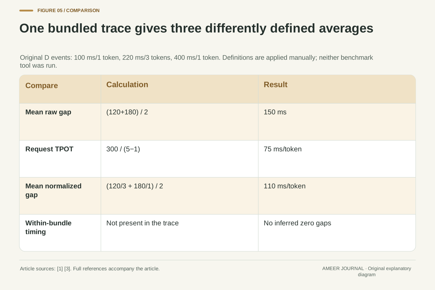
Request D has content events at 100, 220 and 400 milliseconds. The first contains one token, the second contains three and the last contains one. That makes five output tokens in three observed events. Its two visible gaps are 120 and 180 milliseconds, with an average of 150 milliseconds between events.

The per-request token calculation gives a different number. There are 300 milliseconds between the first arrival and completion, and four later tokens. Dividing 300 by four gives 75 milliseconds per later token. The gap average of 150 and the token average of 75 both follow from the same trace.

The middle event does not tell us exactly when its three tokens were generated. We know when the bundle arrived. We should not create extra zero-length arrival gaps and pretend those were separate observations. The vLLM benchmark guide makes this distinction for outputs that bundle tokens, including speculative decoding [1]. Our bundle is simply declared; it does not prove that speculative decoding or any other particular mechanism produced it.

For D, let event arrivals be (100,220,400) ms and event token counts be (1,3,1). The total count is N_D=5, TTFT_D=100 ms and L_D=400 ms. The two inter-output gaps are (120,180) ms, yielding the event-gap mean 150 ms. Request-level TPOT is (400−100)/(5−1)=75 ms/token.

The equivalence between a mean event gap and TPOT used within A, B and C no longer holds because event count differs from token count. The pinned vLLM CLI definition retains only actual stream gaps and does not insert zero-duration samples for extra tokens in an output [1]. This changes the observation count, not the arrival timestamps.

A chunk arrival supplies no intra-chunk generation timestamps. Although multiple tokens become available to this client at the same observed event, that is not evidence that their internal generation intervals were zero. Our calculation needs only the declared event times and counts. It neither reconstructs an engine schedule nor identifies whether server batching, transport buffering or an application choice created the bundle.

A second documented calculation adds another useful comparison. NVIDIA’s GenAI-Perf README defines its inter-token value using the gap before a response divided by the number of generated tokens in that later response [3]. Apply that rule manually to D. The 120-millisecond gap is followed by three tokens, giving 40 milliseconds per token. The 180-millisecond gap is followed by one token, giving 180.

The ordinary average of those two response-level values is 110 milliseconds. We now have three answers for D: 150 between observed events, 75 from its whole post-first-token duration, and 110 from averaging the two normalized response values. Each result has a different denominator or weighting rule.

This is a comparison of written definitions, not a run of either tool. The NVIDIA README also says GenAI-Perf is being phased out [3], so its presence here should not be read as a current tool recommendation. When comparing an existing report with a new one, retain the tool version, formula and sample unit. Matching labels alone cannot establish that the reported numbers measure the same quantity.

The retained native NVIDIA metrics table defines an inter-token observation as an inter-response interval divided by the latter response’s generated-token count, with one value per response per request [3]. For the two post-first events of D, the manually derived observations are 120/3=40 and 180/1=180 ms/token. Their equally weighted mean is 110 ms/token.

That differs from the vLLM-style raw event-gap mean of 150 ms and the request-amortized TPOT of 75 ms/token. Weighting NVIDIA’s two normalized values by their respective later-token counts would give (3×40+1×180)/(3+1)=75, but the equal-response average gives 110. Naming the weight explicitly explains the difference without claiming one formula is erroneous.

No GenAI-Perf output file or vLLM measurement was produced. The source README is retained with its current phase-out notice; the article uses its documented definition as a concrete example of terminology differences. It makes no claim about a successor tool’s behavior. The comparison should be associated with these exact definitions and retrieved documents, rather than generalized to every historical release, backend or similarly named metric.

Request E sends its only token at 90 milliseconds and completes at that same time. Its first-token time and total time are both 90 milliseconds. There is no gap between two token events because a second event never occurs.

Trying the later-token formula produces zero divided by zero: no elapsed time after the first token, divided by no later tokens. That has no defined mathematical value. It does not establish that the server generates tokens instantaneously. It tells us that this request supplies no later-token interval for the measurement we chose.

The vLLM version 0.31.0 metrics documentation records an implementation difference: its server histogram uses zero for requests with no more than one generated token, while its benchmark excludes those requests from its token-time statistics [2]. Such handling affects a summary’s population. We keep E separate from the three-request averages above and report why. A displayed zero, an absent value and an excluded observation should not be assumed to mean the same thing.

E has one content arrival at 90 ms, N_E=1, TTFT_E=90 ms and L_E=90 ms. Its gap sequence is empty. Substituting into TPOT=(L−TTFT)/(N−1) yields 0/0, which is undefined. No positive or zero post-first-token rate can be inferred from that expression.

The pinned vLLM metrics documentation says its server request-TPOT histogram records zero for N≤1, whereas vllm bench serve excludes such requests from its TPOT statistics [2]. This is a documented reporting convention, not a resolution of the undefined quotient. A mean that includes stored zeros can therefore differ from a mean that excludes the same requests even if every multi-token request is unchanged.

Our A/B/C request mean and pooled gap mean include only their explicitly defined observations. E is not inserted as a zero and does not contribute an invented gap. In a real comparison, retain counts of excluded and conventionally encoded records. Without that population information, a changing mix of short responses could alter a dashboard average without demonstrating any change in the timing of comparable generation intervals.

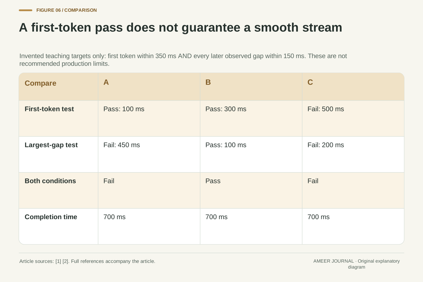
For this exercise only, invent two requirements: the first token must arrive within 350 milliseconds, and no later observed gap may exceed 150 milliseconds. These are teaching thresholds, not recommended limits for a real product or evidence about human comfort. Apply both to A, B and C.

A passes the first condition because it starts at 100 milliseconds, but fails the gap condition because of its 450-millisecond pause. B passes both: its first token arrives at 300 and its largest gap is 100. C fails both because it starts at 500 and has a 200-millisecond gap. Exactly one of the three traces passes the combined rule.

A first-token-only report would count A and B as successes. A completion-only rule set at 700 milliseconds would count all three. The different counts follow from different questions. Decide which events matter, how to combine the conditions and how to handle missing intervals before looking at the result. Our tiny constructed set illustrates those choices; it cannot establish a service’s reliability.

Define an illustrative predicate P_r=[TTFT_r≤350 ms] AND [max(g_r)≤150 ms] for r in {A,B,C}. A evaluates to true AND false, B to true AND true, and C to false AND false. Consequently, sum(P_r)=1 over these three declared requests.

The first-arrival predicate alone passes two of three; the completion predicate L_r≤700 ms passes all three. These outcomes are exact finite counts under different definitions of success. They are not interchangeable service-level statistics, confidence estimates or recommendations for a production SLO. In particular, three constructed traces do not support a claim of 99th-percentile performance.

The predicate is deliberately scoped to requests with nonempty observed gap sequences. It does not silently define max(empty) for E or transfer a token-gap threshold to an unspecified bundled-event measurement. Before using a similar rule on a real dataset, specify its measurement unit, missing-value policy and treatment of failed or canceled requests. Otherwise the denominator and the meaning of a pass can change while the displayed condition appears unchanged.

A’s final pause is real within our invented arrival record, but the record gives no cause. The server might not have produced more content yet, or content might have been delayed elsewhere. The trace does not distinguish those possibilities. Calling the whole pause model time would add information that was never measured.

The vLLM metrics design names separate engine events for entering a queue, being scheduled and producing new tokens [2]. Those timestamps support questions that client arrivals alone cannot answer. If a real investigation needed to separate queue waiting from later work, it would need suitable server evidence connected to the same request.

Likewise, a display problem needs display evidence. Recording arrival at an application boundary is different from recording when the reader sees the text. Keep those timelines distinguishable, and check that any clocks being compared are compatible. Here we intentionally stop at the client boundary. The honest conclusion is that A contains one long observed gap, while the responsible component remains unknown.

Our observables determine arrival intervals, not an internal latency decomposition. A mapping from one client gap to server execution time would require additional assumptions about buffering, scheduling, transport and application processing that are absent from the fixture. No causal component can be assigned the 450 ms interval from these records alone.

The vLLM design documents engine QUEUED, SCHEDULED and NEW_TOKENS events and explains that its frontend cannot see all relevant scheduling boundaries [2]. That is a concrete example of why internal phase measurements need appropriate instrumentation. The document also distinguishes aggregate metrics from traces that follow individual requests. Neither observation makes our client-only record a server trace.

A useful diagnosis would associate compatible timestamps and identifiers across the actual boundaries being investigated, preserving what each event means. It would also state whether completion includes a trailing protocol event after the last content token. Our assumption that those boundaries coincide removes that complication from the arithmetic; it does not prove that deployed systems behave identically. The source describes its own instrumentation, and the article does not prescribe a universal phase decomposition for every model server.

A useful report should let another reader reconstruct its numbers. For these examples, that means retaining each request’s send time, event times, token counts per event and completion boundary. It also means saying that the times are invented. A long list of precise values is not a substitute for an actual measurement.

If you collect a real trace later, record which tool and version produced it, how output tokens were counted and which requests entered each summary. Keep the first-response definition separate from any screen-rendering measurement. Record failures and exclusions so a faster-looking average cannot hide a changed set of completed requests.

For our constructed traces, the findings are clear: equal finishing times can hide different pauses; request and gap averages can differ; bundled tokens change the relationship between events and tokens; and a single-token request has no later-token average. None of this identifies the best model. It gives you a way to read a latency claim closely enough to understand what was measured and which experience its number actually describes.

The reproducible fixture consists of ordered event timestamps, event token counts, request-relative send origins and declared completion boundaries. The derivations additionally specify gap construction, TPOT eligibility, aggregation weights and the scope of the illustrative pass predicate. The retained exact arithmetic uses rational values where needed, including 400/3 ms for the pooled A/B/C gap mean.

A later empirical comparison would require actual workload and configuration evidence, such as input and output count conventions, model and serving versions, sampling settings, load boundaries and failures. These are fields to document for that experiment, not claims that the current exercise controlled or measured them. Since the fixtures lack a shared global workload interval, summing their tokens cannot establish system output throughput.

The demonstrated conclusions concern identifiability and aggregation: event lists contain information absent from totals; a mean of products differs from a product of means; response normalization changes weights; and a reporting convention can conceal an undefined per-request quotient. Preserve the raw observations and the declared formula together. That makes a result reproducible while keeping claims about hardware, software causes and user experience within the boundaries of the evidence actually collected.