What you’ll take away
- Weight storage, compute precision, activation precision, and scale metadata are separate choices; a single bit-width label does not describe all four.[1][2]
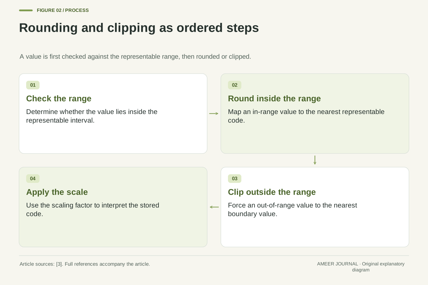
- Rounding moves values to the nearest representable code, while clipping forces out-of-range values to the boundary, so the two error mechanisms must be analyzed separately.[3]
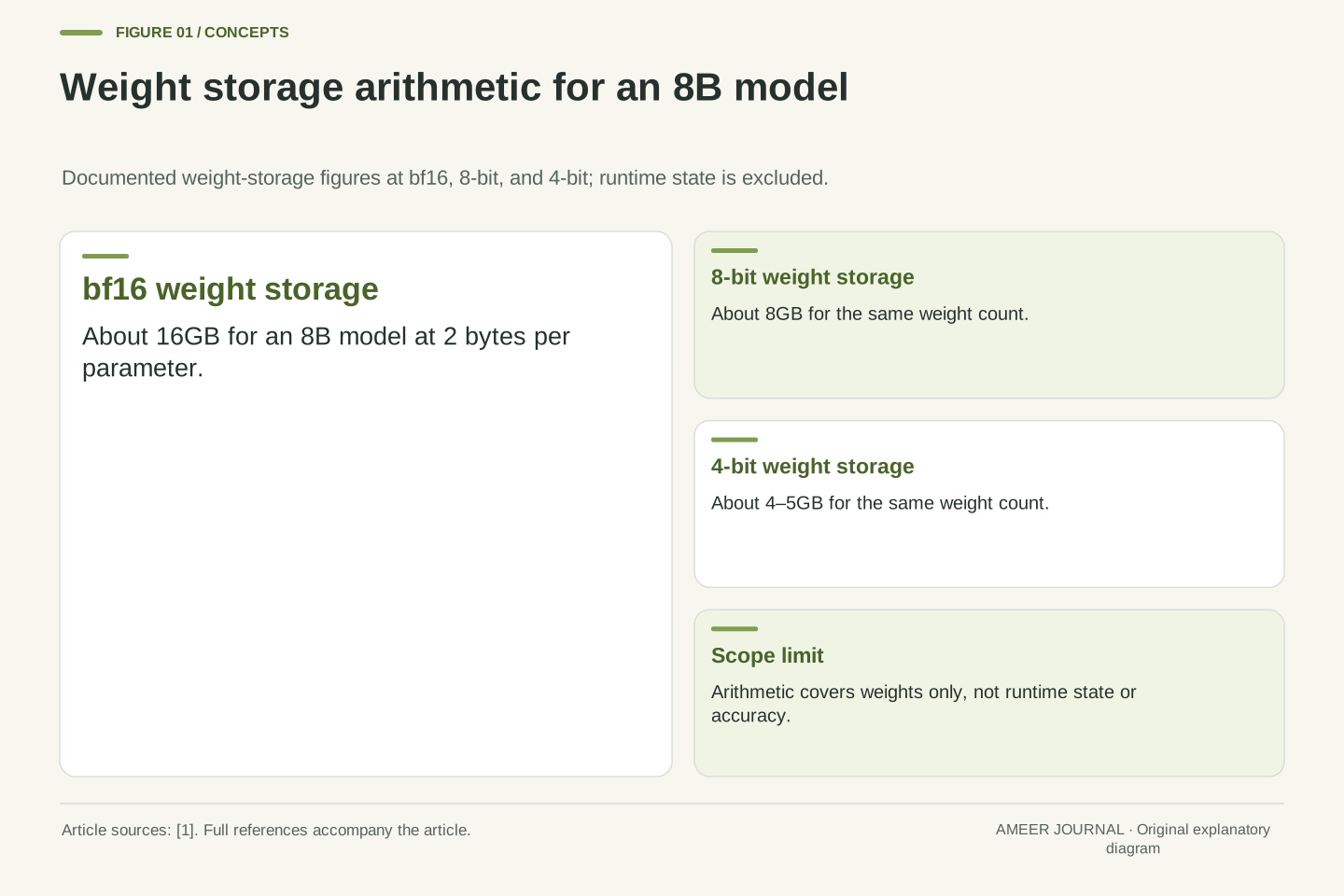
- Storage arithmetic for an 8B model—about 16GB at bf16, 8GB at 8 bits, and 4–5GB at 4 bits—describes weights only and does not establish accuracy or speed.[1]
- Outliers and sensitive computations justify selective higher precision, as in the documented outlier threshold and critical-computation handling for 8-bit quantization.[2]
- Format choice should follow the tensor distribution and the deployment path, not a product name or a bit count alone.[2][3]
The question low-bit quantization actually answers
Low-bit quantization asks a narrower question than it first appears to ask. It does not ask whether a model can be made smaller in every respect, or whether every part of a model should use the same number of bits. It asks which numbers can be represented with fewer bits, where those numbers are stored, and what error that representation introduces when the numbers are used again.[1]
That distinction matters because a model contains more than a single list of weights. It also contains activations, which are the intermediate values produced while the model runs, and metadata, which helps software interpret the stored numbers. A method may compress one of these categories while leaving another at higher precision. Reading a bit-width label as a description of the whole system therefore hides the most important design choices.[1][2]
The useful question is consequently not simply “Is this 4-bit or 8-bit?” It is “What is 4-bit or 8-bit, what remains at another precision, and how are the compressed values restored or used?” Once those questions are separated, the tradeoff becomes clearer: fewer bits usually reduce weight storage, but they can cost accuracy, and different methods balance memory, speed, and accuracy differently.[1]
Low-bit quantization is a family of representation choices rather than a single transformation. The central question is which tensors are mapped to a lower-precision code, whether that mapping is applied to persistent weights, transient activations, or both, and how the resulting codes are interpreted during computation. A bit-width label alone does not specify the tensor scope, the numeric format, the grouping granularity, or the precision used for arithmetic.[1][2]
This separation is essential because persistent storage and runtime computation are distinct resources. A checkpoint may store packed low-bit codes while the runtime expands those codes to a wider compute type before multiplication, or it may execute operations directly in a low-precision format when the hardware and software support it. Conflating storage precision with compute precision therefore produces incorrect expectations about both memory use and numerical behavior.[2][3]
The appropriate evaluation is thus multidimensional. One must identify the quantized tensors, the numeric format, the scale and offset metadata, the dequantization or native compute path, and the tensors deliberately excluded from quantization. Only then can the accuracy cost be interpreted, because each method makes a different tradeoff among memory, speed, and accuracy rather than optimizing all three simultaneously.[1]
Four things not to merge: weights, compute, activations, and metadata
Weights are the learned numbers stored in a model checkpoint. Quantization most commonly targets these weights because they are persistent and can be packed before the model is loaded. In one documented loading pattern, a full-precision checkpoint is quantized as it loads, while in another the checkpoint is already quantized and the stored configuration identifies the method.[1]
Computation precision is different. It describes the format used when arithmetic is performed. A 4-bit stored weight, for example, may be converted to a wider type for computation, and a configuration can specify a separate compute data type. The bitsandbytes documentation gives bf16 as a possible compute type for a 4-bit load, which shows that storage and computation need not match.[2]
Activations are the values created during a forward pass, and scale metadata is the extra information needed to interpret compressed codes. Some methods quantize activations as well as weights, while others preserve higher precision for sensitive computations. A reader who merges these four categories into one label will miss why two models with the same nominal bit width can behave differently.[1][2][3]
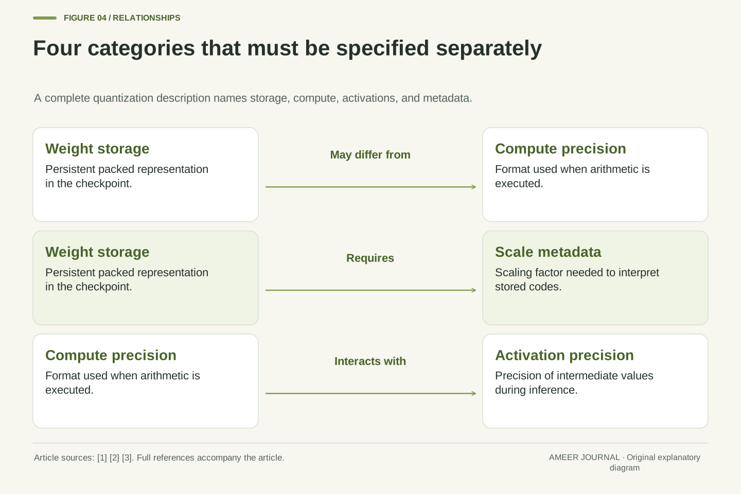
Four categories should be kept analytically distinct. First, weight storage concerns the persistent representation of learned parameters in a checkpoint. Second, computation precision concerns the format in which multiply-accumulate operations and related arithmetic are executed. Third, activation precision concerns intermediate tensors produced during inference. Fourth, scale metadata concerns the parameters—such as a scaling factor—that map integer or low-precision codes back to approximate floating-point values.[1][3]
These categories can be varied independently. A runtime may store weights in a packed 4-bit format, dequantize them to bf16 for computation, keep normalization modules in the default floating-point type, and quantize activations only in selected layers. The bitsandbytes documentation explicitly notes that non-linear modules such as LayerNorm default to a separate dtype and can be changed independently, demonstrating that a quantized linear layer does not imply a uniformly quantized network.[2]
Metadata is not an implementation footnote. In a symmetric scheme, quantized and floating-point representations are related through a scaling factor, so the factor is part of the numerical representation rather than optional documentation. If the scale is missing, ambiguous, or applied at the wrong granularity, the stored codes cannot be interpreted correctly even when the codes themselves were produced accurately.[3]
Storage arithmetic: what fewer bits do and do not prove
The basic storage arithmetic is straightforward. A bf16 value takes 2 bytes, so an 8-billion-parameter model needs about 16 gigabytes for its weights at that precision. The same weight count corresponds to about 8 gigabytes at 8 bits and about 4 to 5 gigabytes at 4 bits in the documented example.[1]
That arithmetic describes weight storage, not the total memory used by a running system. Runtime state, activations, software overhead, and any modules kept at higher precision are not captured by multiplying a parameter count by a bit width. The source material also warns that actual accuracy and latency require measurements, so a storage calculation should not be presented as a benchmark result.[1]
The arithmetic is still useful when its scope is stated honestly. It explains why 8-bit quantization can halve weight memory and why 4-bit quantization can reduce it by roughly a factor of four in the documented bitsandbytes examples.[2] It does not, by itself, prove that a particular model will run faster, fit comfortably on a particular device, or preserve accuracy on a particular task.
Weight-storage arithmetic follows directly from parameter count and bytes per parameter. With bf16 at 2 bytes per parameter, an 8B model requires approximately 16GB for weights; at 8 bits the corresponding figure is approximately 8GB, and at 4 bits it is approximately 4–5GB, with the range reflecting implementation and metadata effects rather than a change in parameter count.[1]
This calculation is a lower-bound style estimate for one component of memory consumption. It excludes activations, temporary buffers, runtime libraries, device fragmentation, and any tensors retained in higher precision. It also excludes the possibility that a runtime dequantizes packed weights into a wider format during execution, in which case peak memory can exceed the size of the packed checkpoint.[1][2]
Accordingly, storage arithmetic should not be converted into an unsourced speed or accuracy claim. The documented overview states that fewer bits cost some accuracy and that methods differ in their memory, speed, and accuracy tradeoffs, while its limitations note that actual accuracy and latency need measurements. A defensible report therefore states the arithmetic, names what it excludes, and treats measured task performance as a separate empirical question.[1]
Rounding and clipping: the two basic sources of representation error
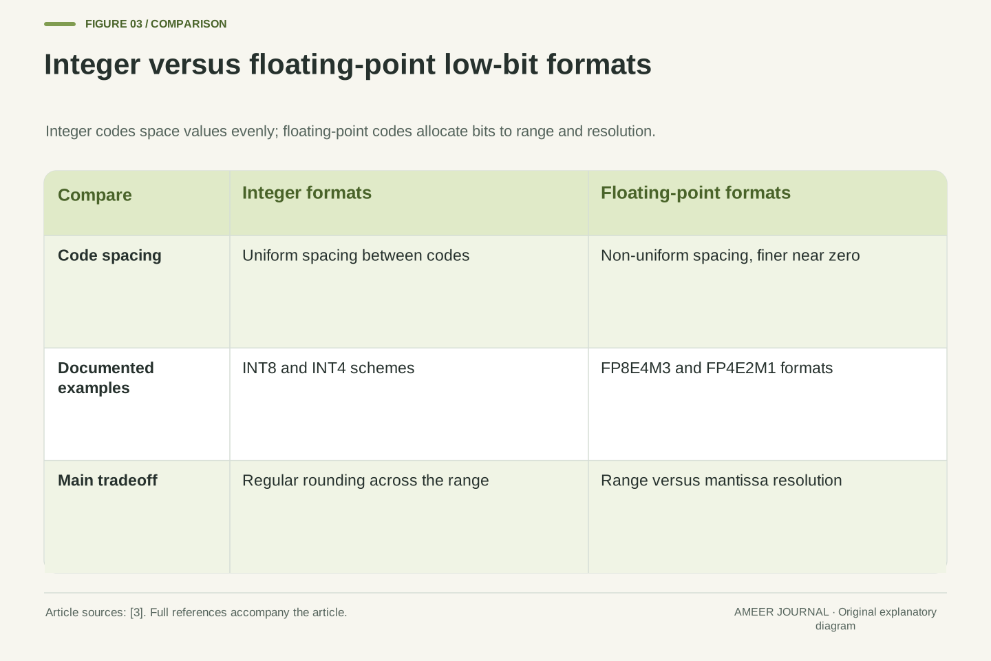
Rounding replaces a value with the nearest representable value. If a format can represent only a limited set of numbers, most original values will fall between two available choices. Rounding moves each value to one of those choices, so the stored value is close to the original but rarely identical. The resulting difference is the rounding error.[3]
Clipping is different. It occurs when a value lies outside the range the format can represent. Instead of choosing the nearest available value inside the range, the system forces the value to the boundary. A large value may therefore be replaced by the largest representable value, which can create a much larger error than ordinary rounding.[3]
Both effects matter, but they fail in different ways. Rounding spreads small errors across many values, while clipping can distort the few values that are unusually large or small. A format with a narrow range may round finely inside that range yet clip important extremes, whereas a format with a wider range may avoid clipping while rounding less precisely.
Rounding and clipping are distinct error mechanisms. Rounding maps a value to the nearest representable code within the supported range, producing an error bounded by half the spacing between adjacent representable values under a nearest-value rule. Clipping maps out-of-range values to the boundary of the representable interval, producing an error that grows with the distance beyond that boundary and is not bounded by the local spacing.[3]
The distinction has practical consequences for format selection. A narrow-range format can provide fine resolution for typical values while saturating on outliers, whereas a wide-range format preserves extremes at the cost of coarser resolution for typical values. Neither property is universally preferable; the correct choice depends on the distribution of the tensor being represented and on which values are functionally sensitive.[2][3]
Error analysis must therefore report more than an average. A small mean error can coexist with a small number of large clipping errors, and those few values may matter disproportionately if they occur in sensitive computations. This is why some 8-bit methods preserve higher precision for critical computations instead of applying a uniform low-precision mapping to every value.[2]
A clearly hypothetical worked example with rounding and clipping
The following example is entirely hypothetical and is designed only to show the arithmetic. Suppose a toy format can represent values in steps of 0.5, from -2.0 to 2.0. Its available values are therefore -2.0, -1.5, -1.0, -0.5, 0, 0.5, 1.0, 1.5, and 2.0. No claim is made that a real model uses this format.[3]
Consider three hypothetical weights: 0.24, 0.76, and 2.4. Rounding 0.24 to the nearest available value gives 0.0, an error of 0.24. Rounding 0.76 gives 1.0, an error of 0.24. The value 2.4 is outside the range, so clipping forces it to 2.0, an error of 0.4. The first two errors come from rounding, and the third comes from clipping.[3]
Now suppose the same three values are multiplied by a hypothetical activation of 3.0. The original products are 0.72, 2.28, and 7.2. Using the rounded or clipped weights gives 0.0, 3.0, and 6.0. The product errors are therefore 0.72, 0.72, and 1.2. The example shows why a modest weight error can become more visible after multiplication, and why the clipped value produces the largest product error in this constructed case.
Consider a purely hypothetical toy codebook with step size 0.5 over the interval [-2.0, 2.0]. The representable set is {-2.0, -1.5, -1.0, -0.5, 0, 0.5, 1.0, 1.5, 2.0}. This construction is an explanatory device only; it is not a claim about INT4, FP4, or any deployed format, and it should not be used to infer the behavior of a real quantization scheme.[3]
Apply nearest-value rounding to the hypothetical weights 0.24, 0.76, and 2.4. The first maps to 0.0 with error -0.24, the second maps to 1.0 with error +0.24, and the third is clipped to 2.0 with error -0.4. The first two errors are bounded by half the step size, 0.25, while the clipping error is determined by the distance outside the interval and would grow if the original value were larger.[3]
Multiplying each weight by a hypothetical activation of 3.0 gives original products of 0.72, 2.28, and 7.2, and quantized products of 0.0, 3.0, and 6.0. The corresponding errors are -0.72, +0.72, and -1.2. The example demonstrates error propagation through a single multiplication, but it does not model accumulation across many terms, correlations between errors, or the nonlinear effects that can occur in a full network.
Scales, grouping, and why metadata is part of the format
A low-bit code is useful only when software knows how to interpret it. In a symmetric quantization scheme, activations and weights are mapped to values centered around zero, and the transformation between quantized and floating-point representations typically involves a scaling factor.[3] The scale is therefore part of the representation, not a decorative label attached to it.
Grouping determines how widely one scale is shared. A single scale for a large tensor is simple, but it must accommodate the full range of that tensor. Separate scales for smaller groups can adapt to local ranges, yet they require more metadata. The tradeoff is between a compact representation and a representation that can follow local variation in the data.[1][3]
Nested quantization illustrates that metadata itself can be compressed. In the documented bitsandbytes feature, a second quantization of already quantized weights saves an additional 0.4 bits per parameter at no additional performance cost according to that documentation.[2] The example should not be generalized into a universal saving, but it shows that the cost of representing scales belongs in the overall accounting.
In symmetric quantization, a floating-point value is mapped to a quantized code through a scaling factor, and dequantization applies the inverse scaling to recover an approximation. Because both activations and weights are centered around zero in the documented TensorRT approach, the scaling factor carries the range information that the low-bit code omits. The code and the scale must therefore be treated as a joint representation.[3]
Granularity controls how that scale is shared. A coarse scale shared across a large tensor reduces metadata but forces one range to serve values with potentially different local distributions. Finer grouping allows scales to adapt to local ranges, improving resolution where values are concentrated, but increases the number of scale values that must be stored, transmitted, and applied during dequantization. The optimal granularity is consequently a tradeoff between metadata overhead and representational fidelity.[1][3]
Nested quantization provides a concrete instance of metadata compression. The bitsandbytes documentation describes double quantization as a second quantization of already quantized weights that saves an additional 0.4 bits per parameter.[2] This figure is specific to that documented feature and should not be treated as a general property of all low-bit formats, but it demonstrates that scale metadata can be a first-order component of the storage budget rather than a negligible constant.
Computation precision can differ from storage precision
A common misunderstanding is to assume that a 4-bit checkpoint means every calculation happens in 4-bit arithmetic. Storage and computation are separate choices. A model may store weights in a packed low-bit form and then convert them to a wider type before performing arithmetic, or it may use a low-precision format directly when the hardware and software support it.[2][3]
The bitsandbytes documentation makes the separation explicit by allowing a 4-bit load to specify bf16 as the compute data type. It also notes that changing the compute type from float32 to bf16 can speed up computation in the documented configuration.[2] That statement concerns a specific configuration and should not be turned into a universal speed claim for all hardware.
The practical lesson is to ask two questions instead of one. First, how are the weights stored? Second, in what precision are they used when the model computes? A checkpoint can be small because its weights are packed, while the runtime still performs arithmetic at a wider precision. Conversely, a low-precision compute path may be available only on suitable hardware and software.
Storage precision and compute precision are independent design axes. A packed 4-bit weight representation describes the persistent encoding, whereas the compute dtype describes the format in which arithmetic is executed after any dequantization step. The bitsandbytes configuration for a 4-bit load permits bf16 as the compute dtype, which confirms that a low-bit checkpoint need not imply low-bit arithmetic throughout the network.[2]
This distinction also explains why dequantization is a meaningful operation rather than a bookkeeping detail. Once quantized, a model can be dequantized to the original precision, but the documentation warns that some quality loss may result and that sufficient memory must be available for the expanded model.[2] The expanded representation is an approximation of the original, not a recovery of the exact pre-quantization values.
Hardware and software support constrain which combinations are available. TensorRT documents INT8, FP8, FP4, and INT4 schemes and distinguishes post-training quantization from quantization-aware training, but its support is version-specific and its performance claims require actual measurements.[3] A format that is mathematically well defined may therefore be unavailable, inefficient, or unsupported in a particular deployment stack.
Activations, outliers, and sensitive computations
Activations deserve separate attention because they are created during computation rather than stored as part of the checkpoint. A method that quantizes weights does not automatically quantize activations, and a method that quantizes both must manage the errors in each. TensorRT documents a symmetric scheme in which both activations and weights are mapped to quantized values centered around zero.[3]
Outliers complicate activation quantization. An outlier is a hidden-state value beyond a chosen threshold, and such values are computed in fp16 in the documented 8-bit method. The documentation notes that values are usually distributed around [-3.5, 3.5], but large models can show very different ranges, and quantization works well for values around 5 while performance penalties grow beyond that region.[2]
Sensitive computations are another reason to avoid a uniform rule. The documented LLM.int8() method dynamically preserves higher precision for critical computations to prevent information loss in sensitive parts of the model.[2] Some modules may also be skipped entirely when quantizing them would cause instability. The lesson is that precision should be allocated where the computation is most sensitive, not spread evenly by default.
Activation quantization differs from weight quantization in both lifetime and distribution. Activations are transient tensors whose ranges depend on the input and on preceding computations, so a scale chosen for weights cannot be assumed to suit them. The documented TensorRT symmetric scheme maps both activations and weights to quantized values centered around zero, but that design choice should not be mistaken for a claim that all quantization methods quantize activations in the same way.[3]
Outlier handling illustrates why activation ranges require explicit treatment. In the documented 8-bit method, hidden-state values beyond a threshold are computed in fp16, with a default threshold of 6 and a warning that lower thresholds may be needed for unstable models or fine-tuning.[2] The threshold is therefore a tunable numerical parameter with an accuracy tradeoff: setting it to 0.0 can speed inference while potentially costing accuracy.[2]
Selective precision is the broader principle. LLM.int8() preserves higher precision for critical computations rather than applying naive quantization uniformly, and the skip-modules option allows particular modules to remain unquantized when conversion would cause instability.[2] These mechanisms acknowledge that numerical sensitivity is unevenly distributed across a network, so a uniform bit width is a simplification rather than a principled default.
Comparing formats by tradeoff, not by product name
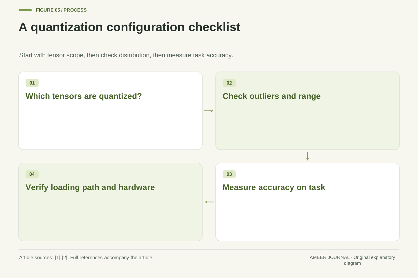
Format names describe different ways of spending a bit budget. INT8 and INT4 use integer codes, while FP8 and FP4 use floating-point codes with exponent and mantissa bits. TensorRT documents FP8E4M3, with 4 exponent bits and 3 mantissa bits, and FP4E2M1, with 2 exponent bits and 1 mantissa bit, alongside INT8 and INT4 schemes.[3] The names alone do not determine which format is best for a given tensor.
Integer formats offer a regular spacing between values, which makes the rounding behavior easy to reason about. Floating-point formats allocate their values unevenly, giving finer resolution near zero and coarser resolution at larger magnitudes. That uneven allocation can be advantageous when values are concentrated near zero, but it also means that range and resolution must be considered together rather than inferred from the bit count alone.[3]
NF4 shows why distribution matters. It is a 4-bit data type adapted for weights initialized from a normal distribution, and the documentation recommends it for training 4-bit base models.[2] For inference, the choice between NF4 and another 4-bit type does not have a huge documented impact, but consistency with the model weights is recommended.[2] A format should therefore be matched to the data it represents, not selected by brand or by bit width alone.
INT and FP formats encode different inductive biases. Integer formats provide uniformly spaced codes, so rounding error is governed by a constant step size across the representable range. Floating-point formats such as FP8E4M3 and FP4E2M1 partition their bits between exponent and mantissa, producing non-uniform spacing that is finer near zero and coarser at larger magnitudes.[3] Neither encoding dominates universally; the appropriate choice depends on the tensor distribution and on whether range or local resolution is the binding constraint.
The exponent-mantissa split makes the tradeoff explicit. FP8E4M3 allocates 4 bits to the exponent and 3 to the mantissa, while FP4E2M1 allocates 2 and 1 respectively.[3] A larger exponent share extends the dynamic range at the expense of mantissa resolution, whereas a larger mantissa share improves resolution within a narrower range. At 4 bits, where only 16 codes are available, this allocation decision is especially consequential because every code assigned to range is unavailable for resolution.
NF4 illustrates distribution-aware format design. It is adapted for weights initialized from a normal distribution and is recommended for training 4-bit base models, while for inference the documented impact of the 4-bit quant type is not huge and consistency with the weights is advised.[2] The general principle is that a format should be evaluated against the empirical distribution of the tensor it encodes, including its outliers, rather than against an abstract preference for integer or floating-point representation.
Choosing a format and checking the result: an actionable checklist
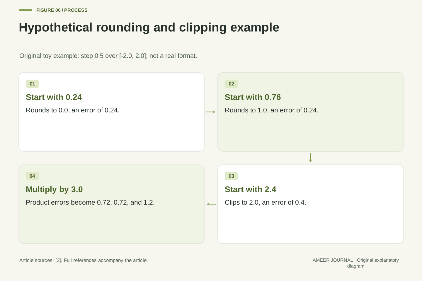
Start by naming the tensor scope. Decide which weights, activations, and modules will be quantized and which will remain at higher precision. Record the storage format, the compute format, and the scale metadata separately, because a single bit-width label does not describe all three.[1][2]
Next, check the distribution before choosing the format. Look for outliers and unusually large values, since those values are the ones most likely to be clipped or to require higher precision. If the method supports an outlier threshold or a skip list, treat those settings as accuracy decisions rather than as minor configuration details.[2]
Then measure the result on the task that matters. Storage arithmetic can show that 8-bit weights take about half the space of bf16 weights and that 4-bit weights take about a quarter, but it cannot show whether accuracy is preserved.[1][2] Compare the quantized model against the unquantized model on representative inputs, and check the sensitive cases rather than relying on an average score alone.
Finally, verify the deployment path. Confirm that the checkpoint format, the loading code, and the hardware support match, and confirm whether the runtime dequantizes weights during execution. A pre-quantized checkpoint is loaded without a quantization config because the method is read from the checkpoint, while a full-precision checkpoint requires a config to quantize during loading.[1] If any of these checks fails, the bit-width label is not a sufficient description of the system.
A defensible selection procedure begins with scope. Enumerate the tensors to be quantized, the tensors to be excluded, the storage format, the compute dtype, the activation treatment, and the scale granularity. This inventory should be recorded before any accuracy claim is made, because two configurations with the same nominal bit width can differ in every one of these dimensions.[1][2]
The second step is distributional analysis. Examine the range and outlier structure of the relevant tensors, since clipping error is governed by values outside the representable interval and rounding error is governed by local spacing. Where the method exposes an outlier threshold, evaluate it empirically: the documented default is 6, lower values may be needed for unstable models, and 0.0 trades potential accuracy for speed.[2]
The third step is task-level validation. Compare quantized and unquantized outputs on representative inputs, with particular attention to cases that exercise sensitive computations or extreme activations. Storage arithmetic—approximately 16GB, 8GB, and 4–5GB for an 8B model at bf16, 8-bit, and 4-bit weight storage respectively—establishes a memory expectation but not an accuracy result.[1]
The final step is deployment verification. Confirm that the loading path matches the checkpoint type, that the required library is installed, and that the hardware supports the chosen format and compute dtype. A pre-quantized checkpoint is loaded without a quantization config because the method is read from its configuration, whereas a full-precision checkpoint requires a config to quantize during loading.[1] Record the measured accuracy and the measured memory separately, and do not substitute one for the other.
Sources & further reading
Explore the references behind this guide. External pages may change after our review.
- Overview · Hugging FaceHugging Face · Accessed 6 Nov 2026
- Bitsandbytes · Hugging FaceHugging Face · Accessed 6 Nov 2026
- Working with Quantized Types — NVIDIA TensorRTNVIDIA · Accessed 6 Nov 2026
Article updated 6 Nov 2026.
Found something we should revisit?
Good explanations get better with thoughtful feedback.