What you’ll take away
- LoRA freezes the pretrained weights and trains only two small low-rank matrices per adapted layer, whose product is added to the frozen weight [1][2].
- The trainable count for one layer is r times the sum of its input and output dimensions, so rank and target-layer choice jointly determine the saving [1].
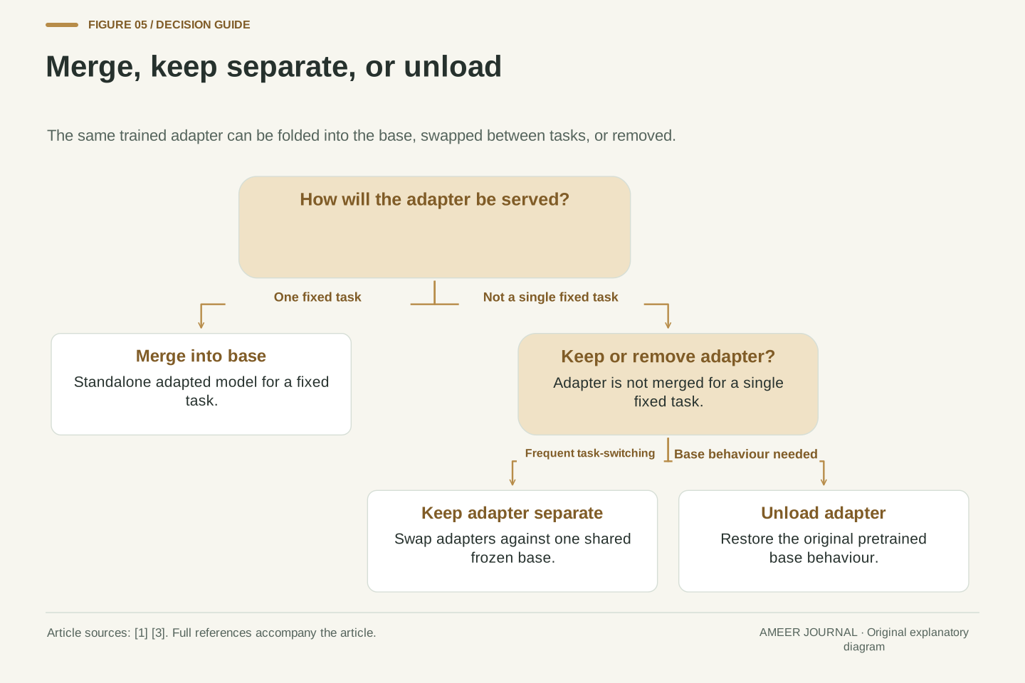
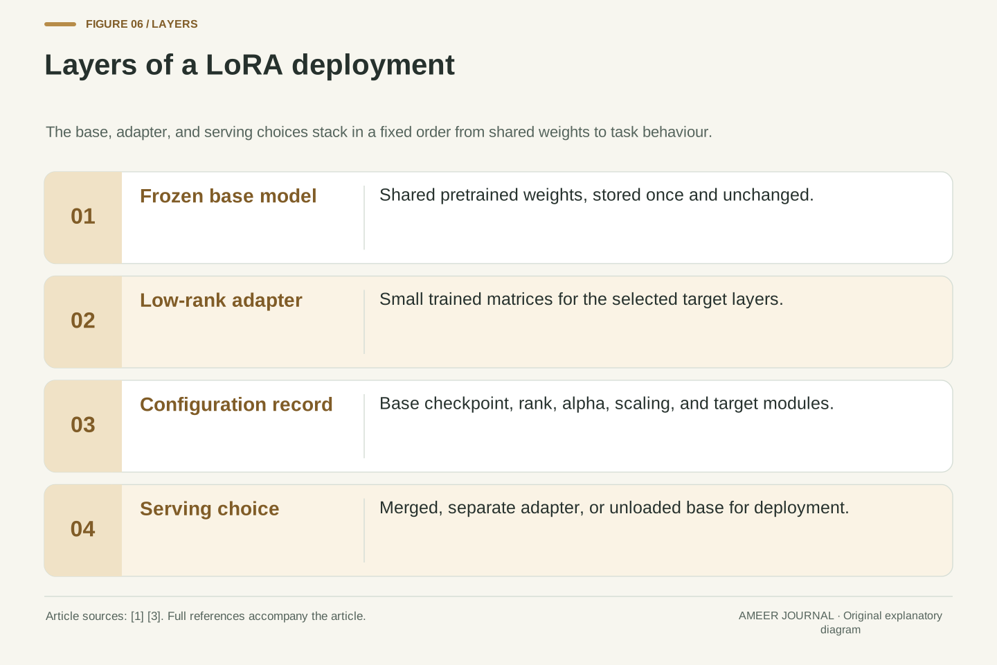
- Adapters can be merged into the base for standalone inference, kept separate for task-switching, or unloaded to restore the original base [1][3].
- Adaptation changes model behaviour through weights, while a document index supplies updatable external content at inference; they solve different problems and should be evaluated separately.
- Reported parity with full fine-tuning is specific to the original experiments, so each new adapter should be compared with its frozen base on held-out task data [1][2].
Start with a frozen base model
Full fine-tuning changes every weight in a pretrained model during training, so each adapted copy must store a complete new set of weights. LoRA takes a different route: the original pretrained weights are kept frozen, meaning they do not receive updates, while only new small matrices are trained to adapt the model to new data [1][2]. This distinction is the whole point of the method, because it separates the shared base from the task-specific change.
The frozen base can then be reused as a starting point for several different tasks. Because the base does not change, multiple lightweight adapters can be built on top of the same pretrained weights, and each adapter can be stored and swapped separately from the large base model [1]. That portability is useful when one base model needs to support several behaviours without keeping a full fine-tuned copy for each one.
Freezing does not mean the model output stays the same. During a forward pass, the frozen weights and the trained adapter weights are combined to produce the adapted result [1]. The base supplies most of the pretrained knowledge, while the adapter supplies a learned correction for the new task, and training concentrates on that correction rather than rewriting the entire network.
In full fine-tuning, the optimiser updates the full pretrained parameter tensor for each adapted layer. LoRA instead treats the pretrained weight matrix as a constant during training and introduces trainable low-rank factors whose product defines the weight update [1][2]. The gradient computation therefore updates only the adapter factors, while the base matrix remains unchanged in memory and in the saved checkpoint.
This parameterisation changes storage and task-switching economics. A single frozen base can serve as a common substrate for multiple downstream adapters, each of which is much smaller than a full model copy [1]. The original authors describe this as freezing pretrained weights and injecting trainable rank decomposition matrices into Transformer layers, greatly reducing the number of trainable parameters for downstream tasks [2].
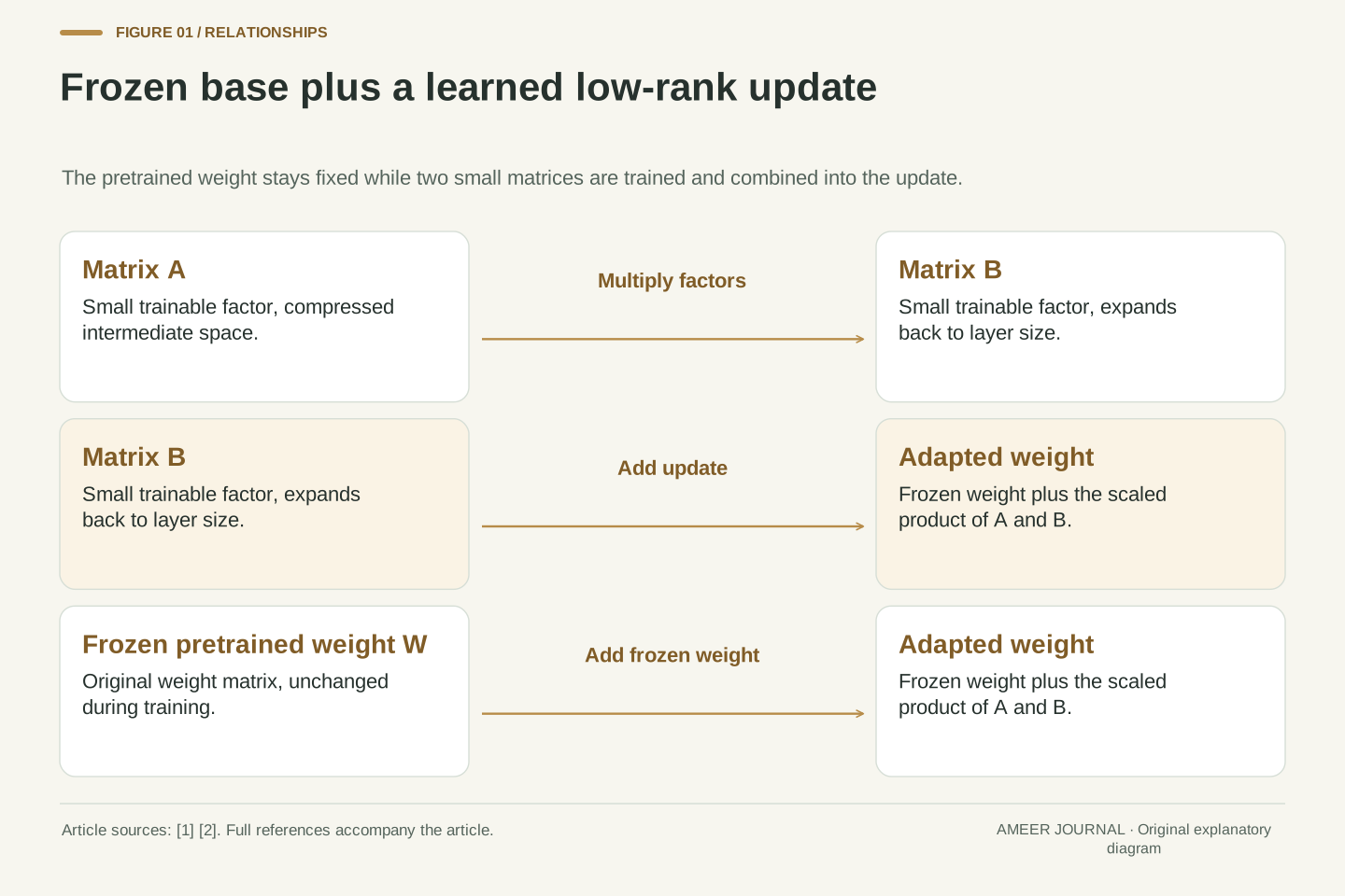
Conceptually, the adapted weight is the sum of the frozen base weight and a scaled low-rank update. The base term preserves the pretrained mapping, and the update term is learned from task data. Because the two terms are combined at inference, the effective model behaves differently from the base even though the base parameters themselves were never modified during training [1].

Why two small matrices can stand in for one large update
A weight matrix in a neural network is a large table of numbers that transforms one set of values into another. If that table has many rows and columns, storing a full change to it would require changing every entry. LoRA represents the change with two smaller matrices instead, a technique called low-rank decomposition, so the number of values that must be learned stays low [1].
The two matrices work as a pair. One matrix first compresses the incoming information into a small intermediate space, and the second expands that compressed information back out to the size needed by the layer. Training adjusts the entries in these two smaller matrices, and their combined effect is the update that is added to the frozen base weight [1].
The word low-rank refers to the size of that intermediate space. A smaller intermediate space means fewer trainable numbers and a more constrained kind of change, while a larger one allows a richer update at the cost of more parameters. The rank, usually written as r, is therefore one of the main controls for how expressive and how economical an adapter is [1].
Let the frozen weight be W, with shape determined by the input and output dimensions of the layer. LoRA does not learn a full delta of the same shape as W. It learns two factors, conventionally A and B, whose product has the same shape as W but whose internal dimension is only r [1]. The update is therefore constrained to lie in a low-dimensional subspace defined by those factors.
The factorisation is the source of the parameter saving. A full update would require as many trainable entries as W contains, whereas the factorised update requires only the entries in A plus the entries in B. When r is much smaller than the layer dimensions, that sum is far smaller than the size of W, even though the product B times A can still produce a full-shaped matrix [1].
Rank also describes a capacity limit. The product of two matrices with inner dimension r cannot have rank greater than r, so the update is restricted to a low-rank correction of the base weight. This restriction is intentional: it biases adaptation toward changes that can be expressed through a small number of directions, rather than arbitrary changes to every entry of W [1][2].
A worked example with dimensions checked
Consider a purely hypothetical layer whose frozen weight matrix W has 8 rows and 4 columns, so it contains 32 numbers in total. This example is invented only to make the arithmetic visible, and it does not describe any real model. If LoRA uses rank r equal to 2, the update is built from two smaller matrices whose shapes must fit together and must match the shape of W when multiplied [1].
The first factor, A, has shape 2 by 4, because it takes the 4 inputs and compresses them into 2 intermediate values. The second factor, B, has shape 8 by 2, because it takes those 2 intermediate values and expands them into 8 outputs. Multiplying B by A gives an 8 by 4 matrix, exactly the shape of W, so the update can be added to the frozen weight without a dimension error [1].
Now count the trainable numbers. Matrix A contains 2 times 4, or 8 numbers, and matrix B contains 8 times 2, or 16 numbers, for a total of 24 trainable numbers. A full update to W would have required 32 trainable numbers, so in this small example the saving is modest. The saving becomes dramatic only when the real layer dimensions are much larger than the chosen rank [1].
Take a hypothetical frozen weight W of shape 8 by 4, containing 32 entries, and set the LoRA rank to r = 2. Factor A is shaped r by 4, or 2 by 4, and factor B is shaped 8 by r, or 8 by 2. The product B A is therefore 8 by 4, which matches W entry for entry, so the adapted weight W plus the scaled product is well defined [1].
The trainable count is the sum of the factor sizes: 2 times 4 plus 8 times 2 equals 24. A full fine-tuning update would train all 32 entries of W. The ratio in this toy case is only 24 to 32, which illustrates an important edge case: low-rank factorisation saves little when the layer is small or when r approaches the smaller layer dimension. The benefit grows as the layer dimensions grow relative to r [1].
The same check generalises. For a weight with output dimension d_out and input dimension d_in, the factors have shapes r by d_in and d_out by r, and the trainable count is r times the sum of d_out and d_in. That formula, rather than any single headline number, is the reliable way to compare an adapter configuration with full fine-tuning for a given layer [1].
Counting trainable parameters before you train
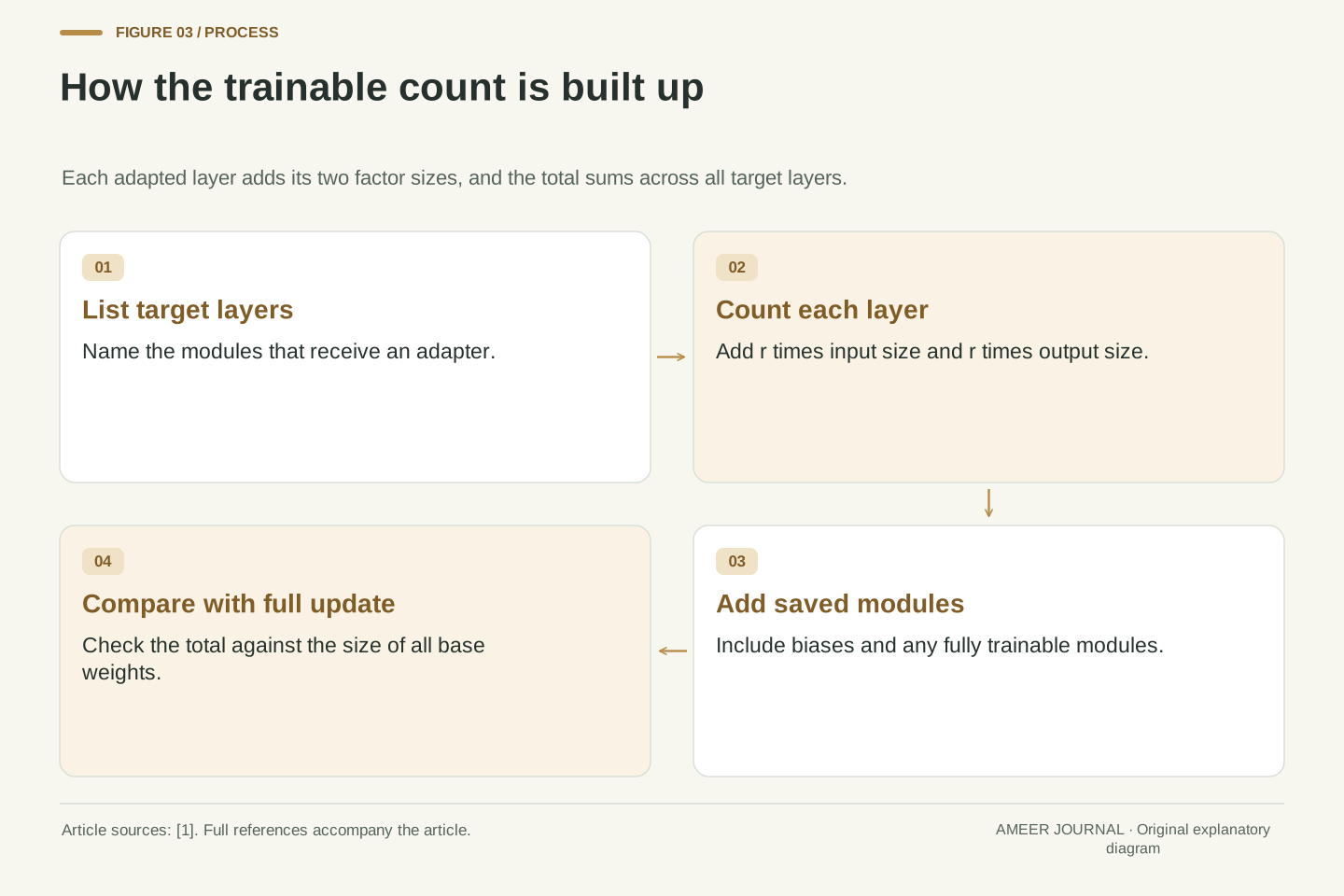
The number of trainable parameters in a LoRA model depends mainly on the rank r and the shape of each original weight matrix that receives an adapter [1]. For every adapted layer, you add the sizes of its two small matrices, and then you add those totals across all adapted layers. Layers without an adapter contribute no new trainable parameters, although the frozen base still has to be loaded for training and inference [1].
This arithmetic explains why target-layer choice matters as much as rank. Adapting only a few layers keeps the trainable count low, while adapting many layers multiplies the count even if each individual adapter is small. A configuration with a low rank applied everywhere can therefore contain more trainable parameters than a higher-rank adapter applied to only one or two layers [1].
It also explains why LoRA checkpoints are small. A saved adapter normally needs to store only the two small matrices for each adapted layer, plus any extra modules that were explicitly made trainable, rather than a complete copy of the base model [1][3]. The base checkpoint is still required to use the adapter, so the saving is in the adapted copy, not in eliminating the base entirely [3].
For one adapted matrix of shape d_out by d_in, the LoRA trainable count is r times d_in plus r times d_out, or r times the sum of the two dimensions. Across a network, the total is the sum of that quantity over every target module, plus any separately trainable modules such as a custom head [1]. The frozen base parameters are excluded from the trainable count, but they still consume memory for storage, loading, and forward computation.
Rank patterns and layer patterns can make this count non-uniform. PEFT allows different ranks for different layers through rank_pattern, and allows selecting which layers are transformed through layers_to_transform and related options [1]. A global rank value therefore does not by itself determine the total; the exact set of adapted layers and any per-layer overrides must be counted as well.
Bias handling is a separate accounting item. The bias option can be set to none, all, or lora_only, which changes whether bias vectors are trained in addition to the low-rank factors [1]. The original implementation likewise allows marking biases as trainable alongside LoRA parameters, with corresponding care needed when saving the checkpoint [3]. Any honest parameter count should state whether biases and saved modules are included.
Choosing which layers receive an adapter
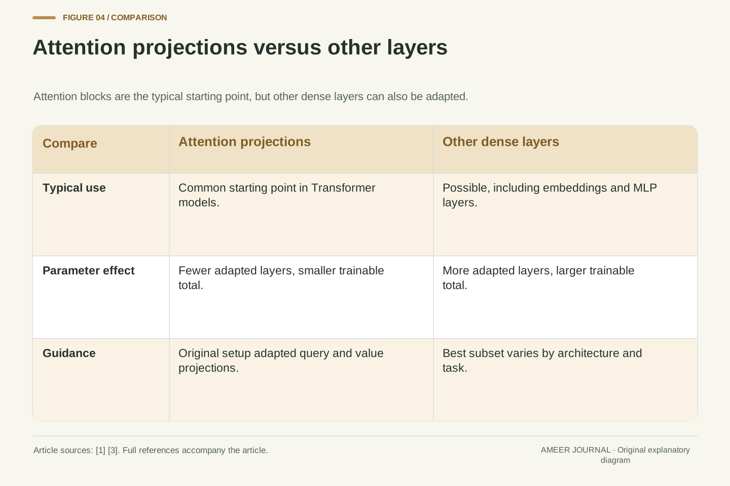
In principle, LoRA can be applied to any subset of weight matrices in a neural network to reduce the number of trainable parameters [1]. In practice, for Transformer models it is typically applied to attention blocks only, because that keeps the method simple and further reduces the number of trainable parameters [1]. The target_modules setting names the modules, such as attention blocks, that receive the low-rank update matrices [1].
The original implementation focused on adapting only the query and value projections in a Transformer, while noting that LoRA can be applied to other subsets of pretrained weights [3]. It also encouraged exploring other configurations, such as adapting embedding layers or multilayer perceptron layers, because the best configuration can vary by architecture and task [3]. There is no universal target set that is correct for every model and every task.
Target choice is therefore an experimental decision, not a default to copy blindly. Adapting fewer layers gives a smaller and more constrained update, while adapting more layers gives the update more places to act but also adds parameters and training cost. The right choice should be tested against the actual task, with the base model and adapter configuration recorded so results can be compared fairly [1][3].
The target_modules parameter selects which named modules receive LoRA factors, and layers_to_transform can further restrict which layers within those modules are adapted [1]. In Transformer implementations, attention projections are the conventional starting point, and the original work used query and value projections as its simple setup [3]. Other dense layers, including embeddings and MLP layers, are possible, but the optimal subset is architecture- and task-dependent [3].
Some implementations complicate target selection. When a single linear layer represents more than one projection, such as a combined query, key, and value projection, the implementation must either split it into separate matrices or use a merged-linear variant that can enable LoRA for selected parts [3]. If the layer is split, the pretrained checkpoint must be modified accordingly, which is an easy place for a silent mismatch between the saved base and the adapted model [3].
Modules_to_save provides another escape hatch for parts that should be fully trainable, typically a randomly initialised custom head for the fine-tuning task [1]. That option can be appropriate when a new output head has no pretrained counterpart, but it also adds a full set of trainable parameters for that module. It should be used deliberately and counted in the parameter total, rather than treated as part of the low-rank update itself [1].
Rank, scaling, and starting values
Rank is not the only control on an adapter. The update is multiplied by a scaling factor during every forward pass, and that factor is fixed at initialisation and depends on the rank [1]. In the original formulation the scaling uses lora_alpha divided by r, while rank-stabilised LoRA instead uses lora_alpha divided by the square root of r, which the documentation says was shown to work better and to stabilise adapters at higher ranks [1].
Starting values matter because training begins from the adapter, not from a random change to the base. By default, PEFT initialises weight A with Kaiming-uniform values and weight B as zeros, which results in an identity transform at the start, meaning the adapter initially adds no change to the base output [1]. A Gaussian initialisation for A, with B still zero, is also available and matches the way some other libraries initialise LoRA weights [1].
These details are easy to overlook because they do not change the shape of the adapter. Two adapters with the same rank and the same target layers can still behave differently if their scaling or initialisation differs. When comparing configurations, it is therefore important to record rank, alpha, scaling mode, and initialisation, not just the number of trainable parameters [1].
The forward computation applies a fixed scalar to the low-rank product, with the default scalar given by lora_alpha over r and the rank-stabilised variant given by lora_alpha over the square root of r [1]. Because the scalar interacts with rank, changing r without reconsidering alpha changes the effective step size of the update as well as its capacity. Rank-stabilised scaling is presented as a way to stabilise adapters and unlock the potential of higher ranks [1].
Initialisation determines the starting point of optimisation. The default PEFT scheme uses Kaiming-uniform for A and zeros for B, producing an identity transform at the start [1]. The Gaussian option initialises A from a Gaussian distribution while keeping B at zero [1]. Setting init_lora_weights to false produces a non-identity starting transform and is described as useful for debugging and testing rather than normal use [1].
A further option, LoftQ initialisation, is intended for use when the base model is quantised, by initialising LoRA weights so that quantisation error is minimised [1]. That option belongs to a combined quantisation and adaptation setup and should not be conflated with plain LoRA on an unquantised base. The key lesson is that scaling and initialisation are part of the method definition, and reports that omit them are incomplete [1].
Merging, unmerging, and unloading an adapter
During training, the small adapter matrices are separate from the base weights. Once training is complete, those weights can be merged into a new weight matrix that is identical to the combined result, so the adapted model can be used as a standalone model [1]. Merging folds the learned update into the base weights, which removes the need to load the base and the adapter as separate pieces during inference [1].
The documentation notes that separately loading a base model and a LoRA model can cause latency during inference, and that merging the adapter weights with the base model eliminates that issue [1]. The original implementation similarly merges LoRA parameters into the pretrained ones when the model is switched to evaluation mode, and unmerges them when training resumes, unless merging is disabled [3]. Merging is therefore a deployment choice about how the final weights are packaged and served.
Merging is not the only option. PEFT provides merge_adapter to merge while retaining the wrapper model for later unmerging or adapter changes, unmerge_adapter to reverse that step, and unload to return the base model without the adapter merged in [1]. Unloading is useful when you want to reset to the original pretrained state, for example when trying out different adapters against the same base [1].
Because the adapted weight is a sum of the frozen base and the scaled low-rank product, the product can be computed once and added to the base matrix after training. The resulting merged matrix is mathematically the same weight that the unmerged forward pass would use, which is why the documentation describes the merged matrix as identical to the combined result [1]. Merging trades a small amount of one-time computation for a simpler inference graph with no separate adapter path [1][3].
The PEFT utilities expose different levels of commitment. Merge_adapter merges while retaining the PeftModel so that unmerging, deletion, or loading different adapters remains possible, whereas unload returns the underlying base model without the active adapter merged [1]. The original library instead ties merging to the train and evaluation modes, merging on evaluation and unmerging on training unless merge_weights is set to false [3].
A merged model is convenient but less flexible. Once the update is folded into the base, switching tasks requires either a different merged copy or an unmerge step, whereas an unmerged setup can swap adapters against one shared base [1]. The choice should follow the deployment pattern: merge for a fixed task served repeatedly, keep adapters separate when task-switching is frequent, and unload when the original base behaviour is required [1].
Keeping several adapters on one shared base
Because the base stays frozen, one pretrained model can support many lightweight adapters for different downstream tasks [1]. Each adapter stores only its small matrices, so a library of task-specific adapters can be much cheaper to keep than a library of full fine-tuned models. The original authors emphasise that this reduces storage for large models adapted to specific tasks and enables efficient task-switching during deployment [3].
Adapters can also be combined. PEFT provides add_weighted_adapter to combine multiple LoRAs into a new adapter using a user-provided weighting scheme [1]. That makes it possible to blend the updates from several adapters, although the result is a new combined adapter whose behaviour still needs to be evaluated rather than assumed to be the sum of the individual strengths [1].
Portability has a limit that is easy to miss. An adapter is only meaningful together with the base model it was trained on, and the original checkpoint must still be available to use it [3]. An adapter trained for one base model, one set of target layers, or one scaling configuration should not be assumed to work with a different base or a different configuration without checking shapes and evaluating the combination [1][3].
The storage argument follows directly from the parameter arithmetic. Each adapter stores the low-rank factors for its target layers, while the shared base is stored once, so the marginal cost of an additional task is the adapter size rather than a full model copy [1][3]. The original work reports this as a way to reduce storage for large models adapted to specific tasks and to enable task-switching without introducing inference latency when adapters are merged [3].
Weighted combination is a separate operation from merging. Add_weighted_adapter creates a new adapter from existing ones according to a user-supplied weighting scheme, which is distinct from merging an adapter into the base weights [1]. The combined adapter remains a low-rank object that can be loaded, merged, or unmerged through the same utilities, but its quality depends on whether the individual updates are compatible [1].
Compatibility is the main risk. Adapters trained on the same base can still interfere if their updates push the shared layers in conflicting directions, and adapters trained on different bases may not even have matching shapes. The safe workflow is to keep adapters versioned with their base checkpoint, target-module list, rank, and scaling settings, and to evaluate each adapter and each combination on held-out task data before deployment [1][3].
Adaptation is not the same as adding a document index
A LoRA adapter changes how a model processes input by changing its weights. A document index, by contrast, stores external documents or passages so that relevant text can be retrieved and shown to the model at inference time. The two approaches solve different problems: adaptation teaches the model a new behaviour or style, while retrieval supplies specific facts or passages that the model can read in context. This section is a general explanation and is not presented as sourced from the LoRA references cited elsewhere in this article.
This distinction matters when choosing a tool. If the goal is to make a model answer in a particular format, follow a particular style, or perform a narrow task more reliably, training an adapter on examples of that behaviour is the relevant approach. If the goal is to answer questions about documents that change frequently, or to cite specific passages, an index that can be updated without retraining is usually the more direct approach, because the knowledge lives outside the weights.
The two can be used together, but they should not be confused. An adapter can learn to use retrieved context in a consistent way, while the index supplies the actual content for each query. Evaluating them separately is important: a model that performs well with retrieved documents may still fail without them, and an adapter that improves style may do nothing to improve factual coverage of new documents.
LoRA modifies the function computed by the network by adding a learned low-rank term to selected weight matrices, so the change is baked into the parameters and applies to every input processed by those layers. Retrieval instead leaves the weights unchanged and changes the input by appending retrieved passages, so the knowledge is supplied per query rather than stored in the parameters. The two mechanisms differ in what is stored, what is updated, and how the system is refreshed. This section is a general explanation and is not presented as sourced from the LoRA references cited elsewhere in this article.
The operational consequences follow from that difference. Updating an adapter requires training data, an optimisation run, and evaluation of the new weights, whereas updating an index requires adding or replacing documents and rebuilding the retrieval structure. An adapter therefore generalises a learned behaviour across inputs, while an index provides exact, updatable content that the model can condition on but does not by itself change the model's underlying behaviour.
Confusing the two leads to predictable failures. Training an adapter on a small set of documents does not create a reliable, updatable memory of those documents, and adding an index does not teach the model a new output format or task behaviour. A sound design states explicitly which part of the problem is handled by weight adaptation and which part is handled by retrieval, then evaluates each part with data that matches its role.
Evaluating an adapter and avoiding common failures
LoRA is reported to perform comparably to full fine-tuning in the original experiments, but that finding is specific to the models, tasks, and configurations studied and should not be read as a guarantee of equal quality for every new task [1][2]. The safe approach is to evaluate the adapted model on held-out data that represents the real task, and to compare it with the frozen base model on the same data. Without that comparison, there is no evidence that the adapter helped at all [1].
Several failures are common and preventable. A rank that is too small may be unable to express the needed change, while a rank that is large, combined with many target layers, can add back much of the parameter cost that LoRA was meant to avoid [1]. Mismatched target layers, a wrong or mismatched base checkpoint, or omitting the pretrained base before loading the LoRA checkpoint can also produce a model that runs but behaves incorrectly. Loading a LoRA-only checkpoint with strict=False after the pretrained checkpoint has been loaded is the expected procedure in the original implementation, not an error in itself [3]. Each of these should be checked before drawing conclusions about the method itself.
A short checklist keeps the work honest. Record the base checkpoint, target modules, rank, alpha, scaling mode, and initialisation; count the trainable parameters including biases and saved modules; verify that the adapter shapes match the base layers; evaluate the base and the adapted model on the same held-out task data; and decide explicitly whether to merge, keep the adapter separate, or unload it for deployment [1][3]. If any step is missing, the result is hard to reproduce or trust.
Evaluation should treat the adapter as a hypothesis about a constrained update. The relevant comparison is between the frozen base and the adapted model on held-out task data, using the same prompts, decoding settings, and scoring procedure for both [1][2]. Claims of parity with full fine-tuning should be tied to the specific experimental setup in which they were observed, rather than generalised into an assumption of zero quality loss for new tasks [1][2].
Edge cases deserve explicit tests. Very small layers or ranks close to the layer dimension yield little parameter saving, as the worked example shows, and combined query, key, and value projections require either splitting or a merged-linear variant with a matching checkpoint [3]. Bias training, modules_to_save, per-layer rank patterns, and weighted adapter combinations all change the effective model and must be included in both the parameter count and the evaluation [1].
The final checklist is therefore: confirm the base checkpoint and target-module list; verify factor shapes against each base weight; record rank, alpha, scaling, and initialisation; count trainable parameters including biases and saved modules; evaluate base and adapted models on identical held-out data; test merging and unmerging round-trips; and version each adapter with the configuration that produced it [1][3]. An adapter that passes these checks is a reproducible, portable change to a frozen base, which is exactly what LoRA is designed to provide [1][2].
Sources & further reading
Explore the references behind this guide. External pages may change after our review.
- LoRA · Hugging FaceHugging Face · Accessed 6 Nov 2026
- LoRA: Low-Rank Adaptation of Large Language Models - Microsoft ResearchMicrosoft Research · Accessed 6 Nov 2026
- GitHub - microsoft/LoRA: Code for loralib, an implementation of "LoRA: Low-Rank Adaptation of Large Language Models" · GitHubMicrosoft / LoRA project · Accessed 6 Nov 2026
Article updated 6 Nov 2026.
Found something we should revisit?
Good explanations get better with thoughtful feedback.